Index
Introduction
This post is the fourth exploring invariance in Machine Learning. In the previous three, I presented the Invariant Causal Prediction, the Invariant Risk Minimization, and the Time Robust Forest. To understand the motivation behind these approaches, I recommend reading the posts about spuriousness and the independent causal mechanism principle.
The Time Robust Tree and Forest (TRF) 1 work was cited in the bibliographic review of the Invariant Random Forest (IRF) 2, which has the same goal but uses a more principled approach to explore invariance.
I will present the IRF algorithm, provide code to reproduce the paper results and run comparisons with a Random Forest (RF) and the TRF.
Invariant Random Forest
Liao, Y. et al. (2024) 2 model the prediction problem with two kinds of features: environmental and stable. Both relate to a target variable over different environments.
The stable features have the same relationship with the target in every environment, but the environmental features are a function of parameters that vary by environment. The idea is to learn only stable features.
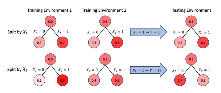
In the image, we see their motivational example. The relationship between \(Y\) and \(X_2\) changes in every environment, while splitting \(X_1\) using the rules \(X_1 = 0\) and \(X_1 = 1\) always provide us the same \(\mathbb{E}[Y \mid X_1]\). It means \(X_1\) is stable, and \(X_2\) is environmental.
The authors introduce the principle that the ratio of the positive and negative classes for a split should be the same in different environments because this is what we expect from the data-generating process of stable features.
Be the stable variables \(S = (S_1, S_2, ...., S_r)\), and environmental variables \(Z = (Z_1, Z_2, ..., Z_t)\). Their generation process, according to \(Y\), is:
\(S \sim P_0(s_1, s_2, ..., s_r), Z \sim Q^e_0(z_1, z_2, ..., z_t), \text{ if } Y=0\) \(S \sim P_1(s_1, s_2, ..., s_r), Z \sim Q^e_1(z_1, z_2, ..., z_t), \text{ if } Y=1\)
Theorem 1 (Liao, Y. et al 2024): For any subset \(D \subset \mathbb{R}^{r+t}\), let \(\tilde{P}_0\), \(\tilde{Q}_0\), \(\tilde{P}_1\), \(\tilde{Q}_1\), be the distribution of \(P_0, Q^e_0, P_1, Q^e_1\) restricted on \(D\), respectively. For a splitting rule \(S_i \leq c\) on \(D\), define the changing rate of positive label as:
\[CR^{1}_{S_i \leq c} = \frac{P(Y = 1 \mid S_i \leq c, X \in D)}{P(Y=1 \mid X \in D)}\]and the changing rate of negative labels as
\[CR^{0}_{S_i \leq c} = \frac{P(Y = 0 \mid S_i \leq c, X \in D)}{P(Y=0 \mid X \in D)}\]These changing rates can be calculated in any environment. Then, using any stable variable as the splitting variable, the ratio between the changing rates of positive and negative labels is invariant across different environments. That is to say, for some \(k\), \(CR^{1}_{S_{i}≤c} / CR^{0}_{S_{i}≤c} = k\) stands for every environment \(e\).
To achieve invariance, they propose a restriction on the split. The \(Q_{m}^{e}\) is the set in the node \(m\) that belongs to the environment \(e\). When the splitting variable \(X_j\) is stable, an invariant across the environment should be:
\[I(Q^e_m, \theta) = CR^1_{X_j} = CR^1_{X_j \leq c}(Q^e_m)/CR^0_{X_j \leq c}(Q^e_m)\]So the optimization becomes:
\[\begin{aligned} &\theta^* = \text{argmin}_{\theta} G(Q_m, \theta), \\ &\text{subject to } I(Q^e_m, \theta) = I(Q^f_m, \theta), \quad \forall e, f = 1, 2, \ldots, E. \end{aligned}\]However, exacting this ratio in every environment for a particular split is a hard, unrealistic condition. So, the authors propose a loss function \(L\) related to it, in which we add a penalty term. The loss is the ratio between the highest and the lowest \(I(Q_m^e, \theta)\) minus 1:
\[L(Q^1_m, ..., Q^E_m, \theta) = \text{max}_{e,f}I(Q^e_m, \theta)/I(Q^f_m, \theta) - 1\]Notice that \(e\) is a specific environment, and \(f\) represents all available environments.
To smooth it:
\[\tilde{CR}^{0}_{X_j \leq c} \propto \frac{|\{(x, y) \in Q^e_{m, l}(\theta) \mid y=0\}| + 0.5}{|\{(x, y) \in Q^e_m(\theta) \mid y=0\}| +1}\]They also provide one for regression, but I won’t explore it in this post.
Here’s the part of the code that performs these operations, making it easier to grasp what is happening.
def gini_invariance_penalty_score(right_dict, left_dict,
                                  invariance_penalty=10,
                                  verbose=False):

    agg_right_dict, agg_left_dict = aggregate_dict(right_dict,
                                                   left_dict)

    # And ugly workaround to use the same function I use for the Time Robust Forest
    overall_gini = gini_impurity_score_by_period({"dummy": agg_right_dict},
                                                 {"dummy": agg_left_dict})[0]

    invariance_loss = invariance_loss_function(right_dict, left_dict)
    if verbose:
        print("Overall_gini: {}, invariance_penalty: {}, invariance_loss: {}".format(
        overall_gini, invariance_penalty, invariance_loss))

    return overall_gini + (invariance_penalty * invariance_loss)

def changing_rate(env_right_dict, env_left_dict, pos_class):
    total_positive = env_left_dict["sum"] + env_right_dict["sum"]
    total_negative = env_left_dict["count"] + env_right_dict["count"] - total_positive

    if pos_class:
        return (env_left_dict["sum"] + 0.5) / (total_positive + 1)
    else:
        return (env_left_dict["count"] - env_left_dict["sum"] + 0.5) / (total_negative + 1)

def invariant(env_right_dict, env_left_dict):

    pos_changing_rate = changing_rate(env_right_dict, env_left_dict, pos_class = True)
    neg_changing_rate = changing_rate(env_right_dict, env_left_dict, pos_class = False)

    return pos_changing_rate / neg_changing_rate


def invariance_loss_function(right_dict, left_dict):
    invariants = []
    for env in right_dict.keys():
        invariants.append(invariant(right_dict[env],
                                    left_dict[env]))

    return (max(invariants) / min(invariants)) - 1
Synthetic data example
I will use the synthetic example from the IRF paper.
\[\begin{align} Y &= \text{Bern}(0.5), \\ X_1 &= |Y \cdot \mathbf{1}_d - C_1| + N_1, \quad C_1 \sim \text{Bern}_d(0.3), \\ X_2 &= |Y \cdot \mathbf{1}_d - C_2| + N_2, \quad C_2 \sim \text{Bern}_d(U_e), \\ N_1, N_2 &\sim \mathcal{N}(0, I_d). \end{align}\]It utilizes a $d$-dimensional Bernoulli distribution where each dimension operates independently. The vector $\mathbf{1}_d$ consists entirely of ones and matches the dimensionality $d$. Additionally, $I_d$ represents the identity matrix of size $d \times d$. For the experiments, I set the parameters as the authors as $U_1 = 0.1$, $U_2 = 0.4$, and $U_3 = 0.7$. The training datasets come from two distinct environments ($e = 1$ and $e = 2$), whereas the testing dataset comes from a third environment ($e = 3$).
Let’s try to reproduce the results displayed in the paper that use \(\lambda={1, 5, 10}\) for the invariance penalty. I use 50 estimators and 10 as the maximum depth. The \(d=5\), and there are 5k examples for every environment. I bootstrap the data five times. The standard deviation is in parentheses.
| Model | Train AUC | Holdout AUC | Train ACC | Holdout ACC |
|---|---|---|---|---|
| IRF ($\lambda=1$) | 0.918 (0.004) | 0.567 (0.011) | 0.836 (0.005) | 0.548 (0.011) |
| IRF ($\lambda=5$) | 0.885 (0.002) | 0.598 (0.005) | 0.801 (0.004) | 0.569 (0.004) |
| IRF ($\lambda=10$) | 0.876 (0.004) | 0.610 (0.009) | 0.791 (0.005) | 0.579 (0.007) |
This reproduction is not explicit in the code provided, but it is trivial to insert these parameters on it.
The results are consistent with the expectation that the higher the penalty, the lower the training performance and the higher the holdout. The magnitude differs from the paper but is not very meaningful. The following comparisons will be interesting since the code base will be the same for the other models.
Profiling the IRF behavior as we change the invariance penalty
To characterize the model behavior regarding the invariance penalty term, I run it for different values for \(\lambda\). I will use 10 as the max_depth and 10 n_estimators and run it 5 times. Regarding the data, I use \(d=20\) and \(n=10k\).
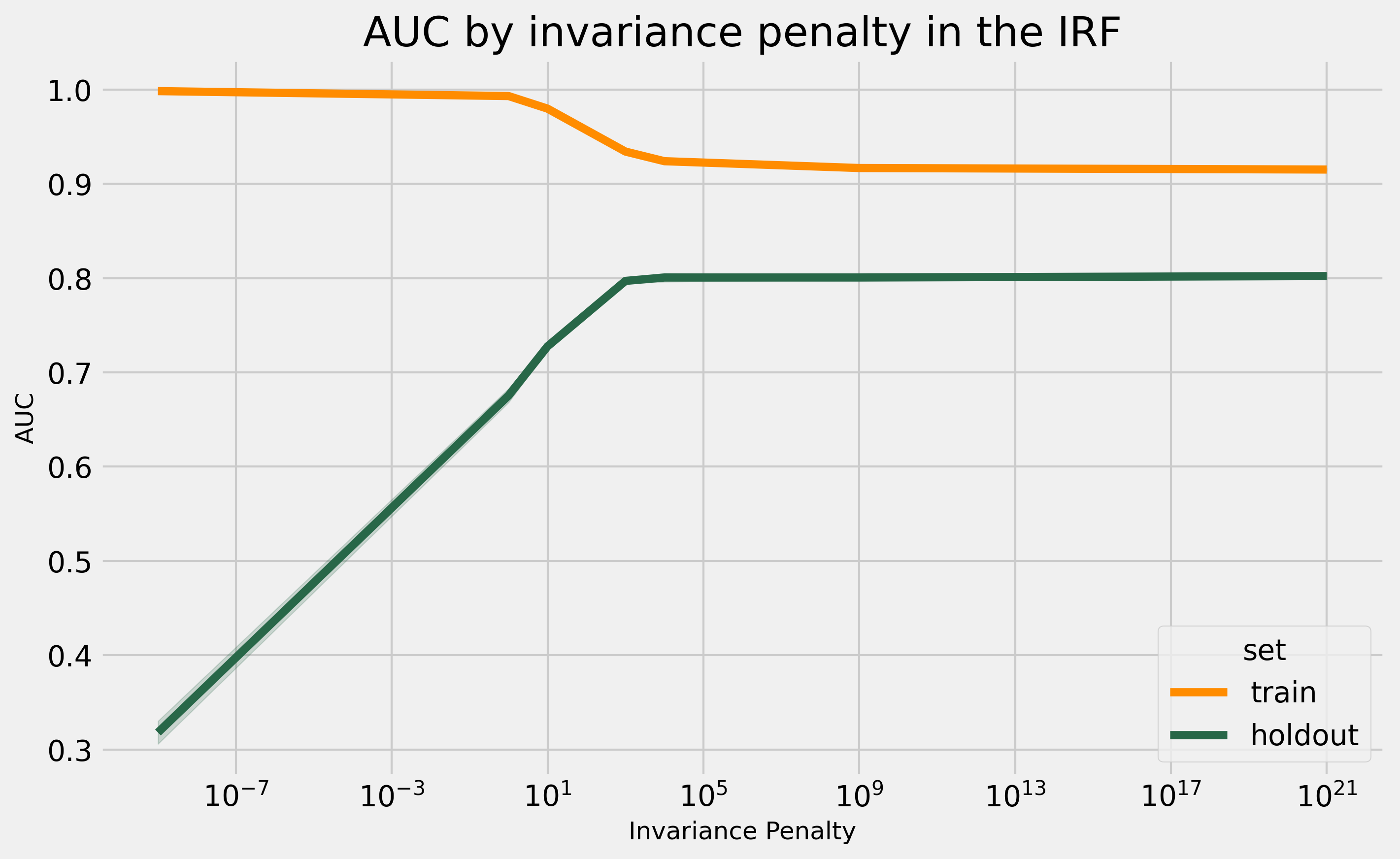
The above plot is quite interesting. Considering all the other parameters fixed, the penalty parameter increases the holdout performance until it saturates. At this point, it mostly looks for variables that satisfy the invariance condition. For regularization terms, we usually expect a quadradic relation. We try to get closer to the maximum, and exceeding it harms the holdout performance. This data is idealized, so I will also run a similar experiment in a real dataset later in this post.
IRF, TRF, and RF on the synthetic example
In this experiment, we want to compare the Invariant Random Forest (IRF), Time Robust Forest (TRF), and Random Forest (RF). We let these models optimize using a random sample of the training environments - this choice is essential. A common alternative approach when the environment information is explicit is to keep one or more out of the training data and use it as the validation set to optimize the hyper-parameters.
For the hyper-parameter optimization, I will fix the number of estimators at 50 while using the following search space for the others:
params_grid = {"n_estimators": [50],
              "max_depth": [1, 5, 10, 15],
              "min_impurity_decrease": [0, 0.0001],
              "min_sample_periods": [1, 5, 10, 100],
              "period_criterion": ["max", "avg"],
              "invariance_penalty": [0, 1, 10, 10e2, 10e3]}
I use the “Env K-fold min-max” 1.
The optimal parameters were:
# RF
{'max_depth': 15,
 'min_impurity_decrease': 0,
 'min_sample_periods': 5,
 'n_estimators': 50}
# TRF
{'max_depth': 10,
 'min_impurity_decrease': 0.0001,
 'min_sample_periods': 10,
 'n_estimators': 50,
 'period_criterion': 'max'}
# IRF
{'max_depth': 15,
 'min_impurity_decrease': 0.0001,
 'min_sample_periods': 10,
 'n_estimators': 50,
 'invariance_penalty': 1000.0,}
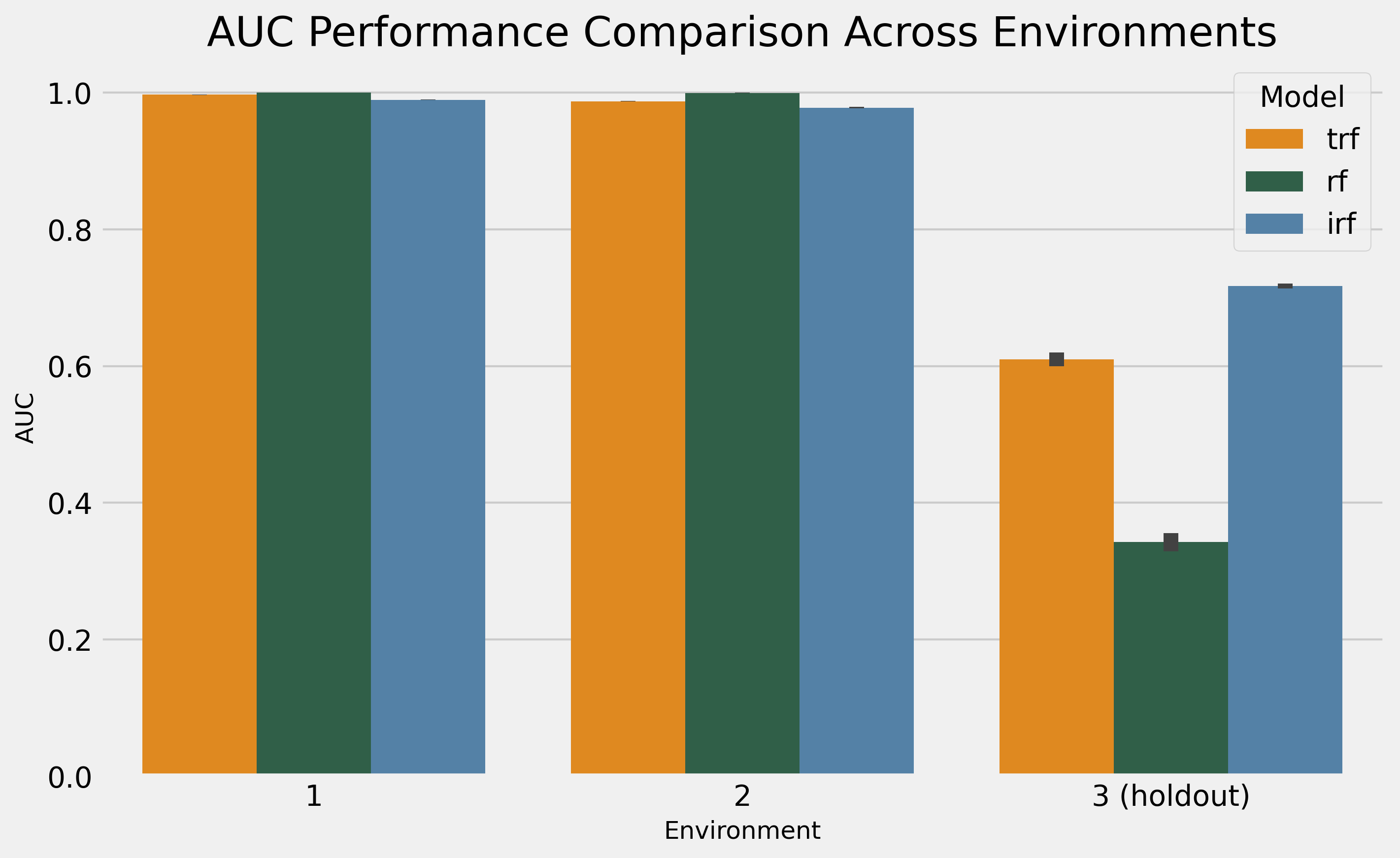
The results show how the RF suffers from the trap both TRF and IRF idealize to solve, while the IRF had a meaningful advantage margin over the TRF, from 0.61 to 0.72. Now, it is time for some real-world data!
Real-world data experiments
I will use the Financial dataset example from IRF’s paper 2.
The dataset contains 5 years of data. The first three years are the training period, and the remaining two are the holdout set, which we wouldn’t have access to at the modeling stage. It differs from the IRF paper since the authors used any three years as training and the remaining as the holdout.
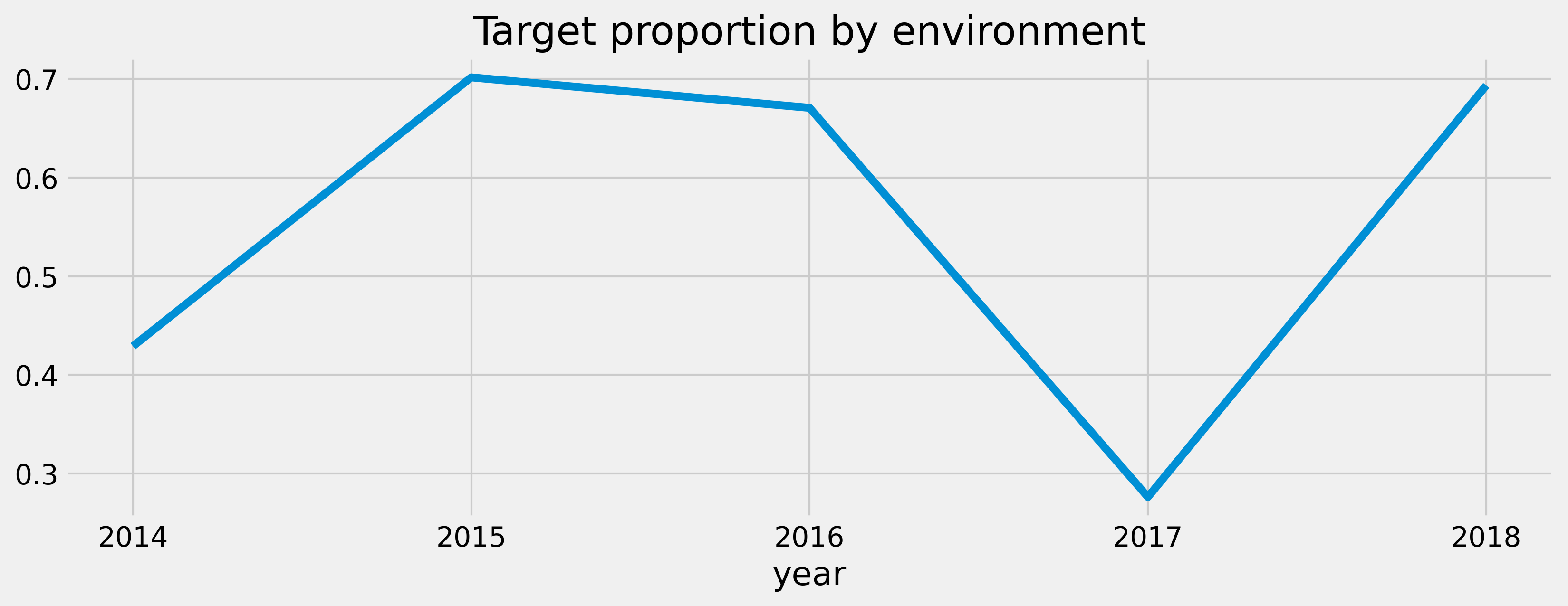
Looking at the target distribution, we see that 2017, one of the holdout periods, behaved weirdly.
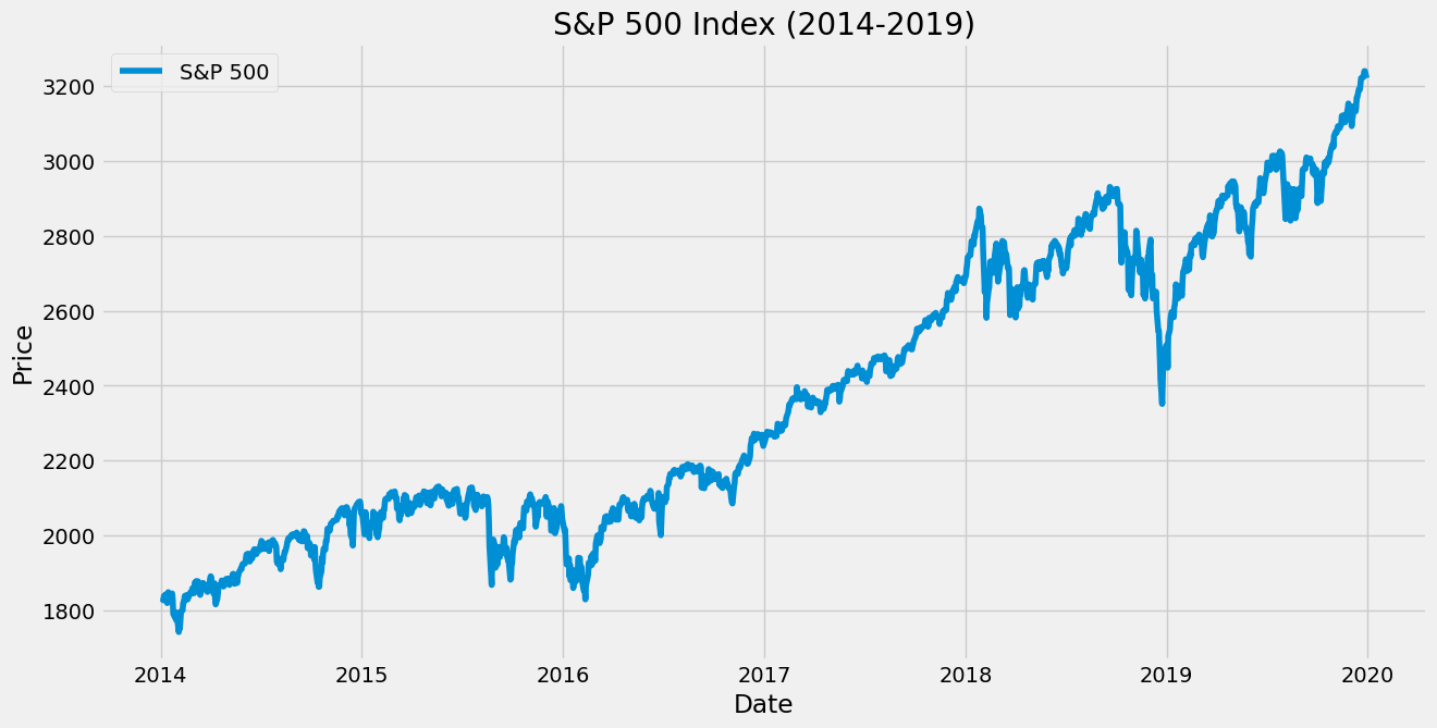
Looking at the S&P 500’s behavior for this period, we can see a significant drop at the end of 2018, which influences the target for 2017 data points and fits the idea that a lower proportion of the stocks in the dataset have a positive label. Since I intend not to understand this dataset in particular, I won’t investigate further.
Ideally, I’d follow the same optimization design from the synthetic data case. However, due to the cost of running it in a real dataset, I will replicate the same hyper-parameters from the synthetic case and bootstrap the data.
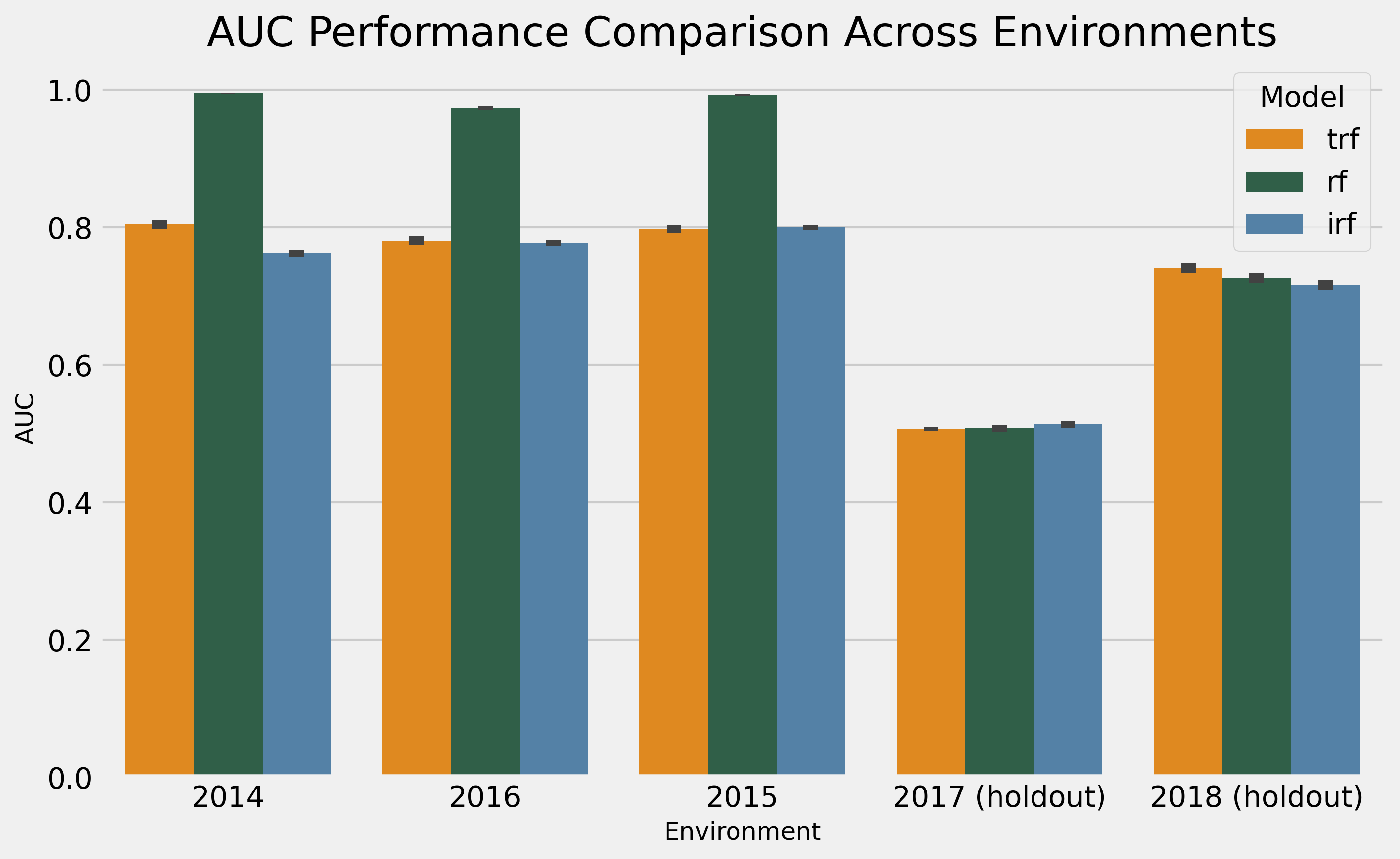
The results show random performance during 2017 for all models, with a slight advantage for the IRF. In 2018, the TRF had a 0.741 AUC, which was a good advantage over the RF (0.726) and the IRF (0.715).
As a second approach, I will optimize the RF using sklearn for speed, replicate the parameters for the IRF and TRF, and use the heuristics I know about them to define the remaining parameters.
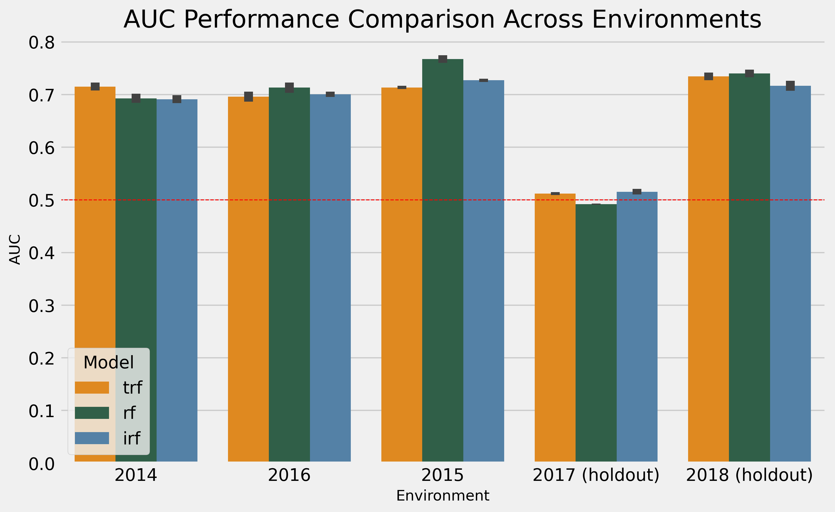
In this case, the RF has a higher performance, which is unsurprising since we optimized for it. The minor tweaks using heuristics for the TRF and IRF were insufficient to make them better than the RF. So, I guess I need to improve my manual optimization skills.
As a last experiment, I will change the invariance penalty in the real dataset to see if it behaves similarly to what we have seen in the synthetic data.
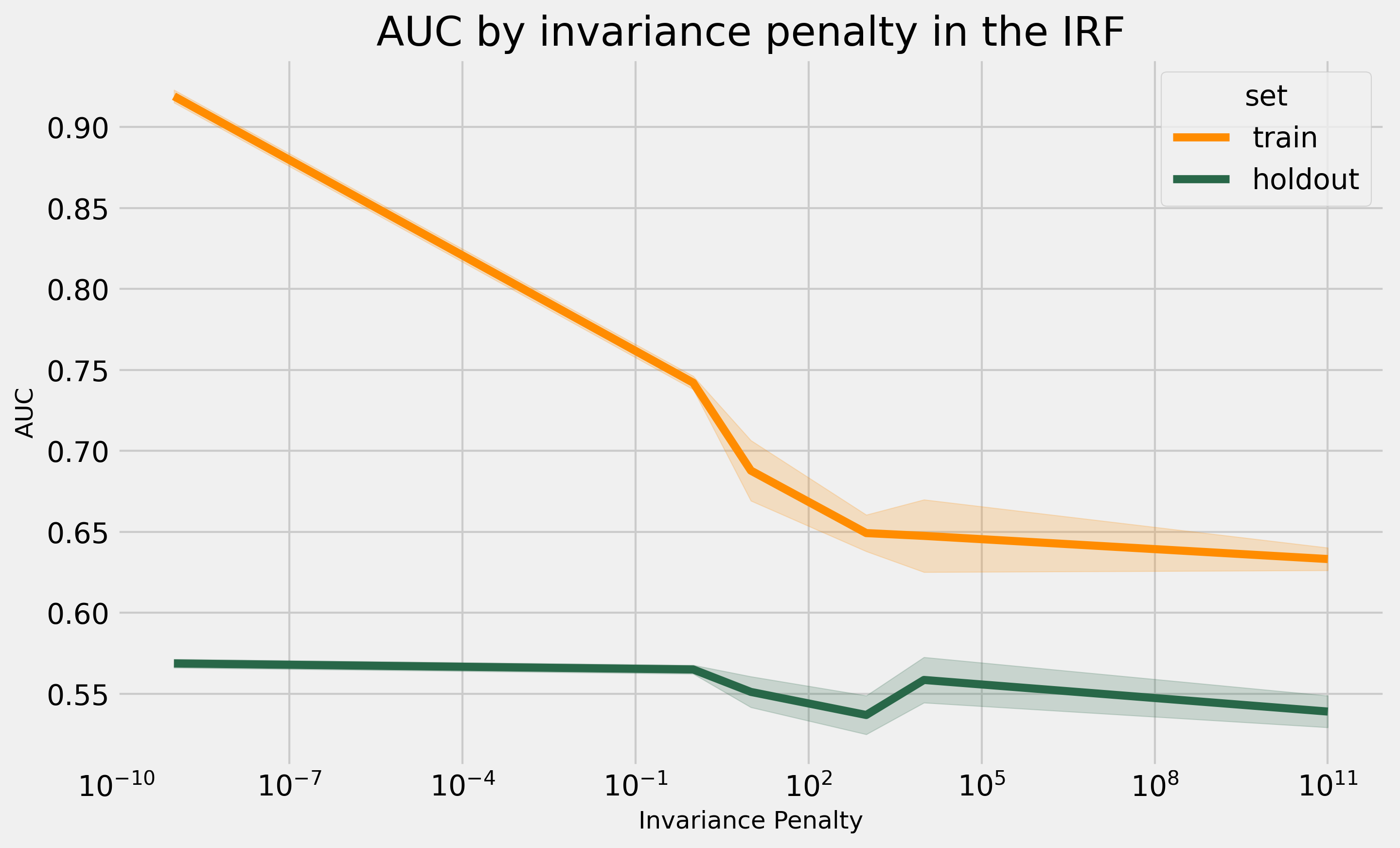
This plot behaves differently than the pattern in the synthetic case. In fact, it tells us that with these hyperparameters, the penalty only harms the holdout performance. However, this is only a single dataset, and more investigation is needed to reach conclusions.
Conclusion
The IRF offers a simple and principle model to explore invariance in tree-based models, which are a very convenient class of predictors. You can see how simple it is to prepare the data for it.
The synthetic data’s performance shows that it can do better than the TRF. For real data, I need more use cases for conclusions. I might give it a try using the same datasets I used for the TRF work or simply keep applying the IRF as I work on new projects and report how it goes.
References
-
Moneda, L., & Mauá, D. (2022). Time robust trees: using temporal invariance to improve generalization. In Brazilian Conference on Intelligent Systems (pp. 385–397). ↩ ↩2
-
Liao, Y., Wu, Q., & Yan, X. (2024). Invariant random forest: tree-based model solution for ood generalization. In Proceedings of the AAAI Conference on Artificial Intelligence (pp. 13772–13781). ↩ ↩2 ↩3