Index

1. Introduction
2. Motivation
3. The algorithm
4. Synthetic example
5. The period-wise performance aggregation
6. The package
7. Conclusion

Introduction

This is the third post of a mini-series exploring invariance in Machine Learning. In the previous two, we presented the Invariant Causal Prediction and the Invariant Risk Minimization. To understand the motivation behind these approaches, I recommend reading the posts about spuriousness and the independent causal mechanism principle.

We will introduce the Time Robust Tree (TRT), a learning algorithm developed during my MSc, advised by Denis Mauá. The algorithms focus on the temporal aspect of spurious relationships to identify correlations that survive the test of time, expecting they are more likely to keep this behavior in future environments and thus result in better generalization.

Motivation

Ideally, we want to learn concepts or models that we can transport to the future with minimal effort. As discussed in the previous posts, one way of achieving such a goal is to ensure invariance to different environments, which are originated by valid interventions in a causal model.

Assume two finite-valued input variables \(X_1\) and \(X_2\), a binary target variable \(Y\), and a time period \(T_{period}\), used to segment the data in different diverse environments. We use three time periods to illustrate, thus \(T_{period}=\{1, 2, 3\}\). Consider the data illustrated in Figure 1.

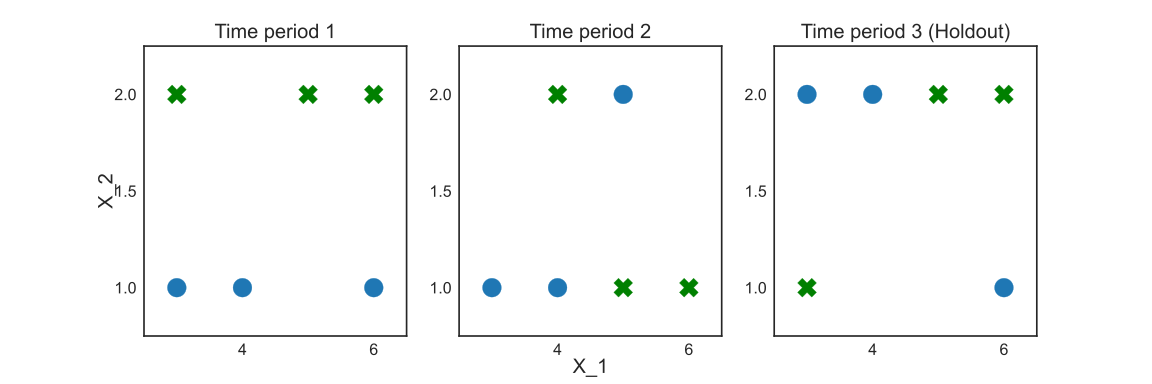
Imagine the data from \(t={1, 2}\) consists in the available training set, while the \(t=3\) comes from the future after deployment. We will call it the holdout set. According to the example, \(X_1\) is mildly predictive and stable. At the same time, \(X_2\) is a perfect predictor at \(t=1\), but its relationship with the target changes in the following periods, representing a spurious correlation or a non-static causal relation that shifted.

Suppose the modeler uses all the available training data. In that case, a typical Decision Tree (DT) inducing algorithm will combine the data from periods 1 and 2 into a single training data set to evaluate the possible splits. In this case, the DT will choose \(X_2 > 1\) as the optimal split.

We use the Area Under the Curve (AUC) to evaluate predictions’ quality. It goes from 0 to 1, and the higher, the better. By learning the \(X_2\) split, the Decision Tree would achieve a 0.83 AUC on training, but a poor result on holdout, 0.50 AUC.

The TRT uses the timestamp information as a hint for diverse environments to inform the learning process and avoid this pitfall.

The Algorithm

A Time Robust Tree is obtained by modifying the standard Decision Tree induction algorithm, using the standard deviation reduction criteria for regression problems and impurity minimization following the Gini impurity for classification problems. These impurity functions are identified as \(L\).

Consider a timestamp column \(T_{stamp}\) representing the data capture time with the exact dimension of the random variables vectors \((X_1, ..., X_d, Y)\), where the \(X\) variables represent inputs and \(Y\) the variable of interest, the target. The time period \(T_{period}\) is an aggregation of sequential examples when ordered by \(T_{stamp}\) using a human-centered concept, like hourly, daily, weekly, monthly, yearly, or simply putting together a fixed number of examples and reducing \(T_{stamp}\) granularity.

Given \(n\) time periods \(T_{period} = t_1, t_2, \ldots, t_n\) in the training set, we find the best split \(s^*\) to divide the examples in \(X_{node}\) into \(X_{left}\) and \(X_{right}\) using the rule \(X_f \leq v_f\) where \(f\) is a feature from all available features \(F\) at a certain value \(v_f\) from all possible values for the feature \(f\) in the training set \(V_{f}\) by applying recursively to every node data \(X_{node}\) until the constraints are not satisfied, being the first node the root containing all the training set, as in Equation \ref{eq:best_split}. Consider the sample size from every period as \(N_t\), the chosen minimum number of examples by period to split as \(\rho\), the maximum depth as \(d\), the minimum impurity decrease as \(g\), and the impurity decrease after the split as \(ID(X_{node})\), which is defined in Equation \ref{eq:period_wise_impurity_decrease}.

The \(\rho\) is a scalar representing the minimum number of examples in every time period to perform a split. The model also accepts the average loss criteria.

For the predictions \(\hat{Y}\), the average from the leaf is taken without any consideration about the time period it belongs, \(\hat{Y} = \frac{1}{|Y|} \sum y_i\).

It is worth isolating in the Equation \ref{eq:period_wise_score} one of the differences from TRT. This period-wise score considers how the model performs in the different periods defined by the user to decide the optimal split. Notice the other difference, the hyper-parameter $\rho$, interacts significantly with this part of the process. Higher $\rho$ guarantees a higher sample in each period for their evaluation regarding the split.

Similarly to the period-wise score, we have the impurity decrease calculation iterating over the periods. The \(L_{before\_split}(X_t)\) gives the impurity measurement in the node before splitting it with a rule, while \(L(X_t)\) gives it after the split. Their contrast informs the decrease, weighted by the number of examples from a particular period in that node and the total available in the sample.

The process is summarized in Algorithm 1. It starts with a call to LearnTimeRobustTree with all the features in \(X\).

Before learning a rule to split the data, there is a condition to stop learning on the maximum depth and the minimum number of examples by period. In CreateSplit, the algorithm learns a split that generates two subsets of the original data, $X_{left}$ and $X_{right}$, for which we call the learning function again and keep splitting until the stop conditions are met. The search for the particular split happens on FindBestSplit, where we discard any split that does not keep the minimum number of examples in every period after applying it and evaluate the best as the one with the lowest score calculated by PeriodWiseScore, which represents the implementation of the Equation \ref{eq:best_split_average}. In case we have opted to use the worst-case score, the PeriodWiseScore would store the score calculated in every period and return the worst case to represent the split quality. Similarly, we calculate the impurity decrease using the PeriodWiseImpurityDecrease, which can use the average value for every period or the worst case.

    \begin{algorithm}
    \caption{Time Robust Tree}
    \begin{algorithmic}
      \PROCEDURE{LearnTimeRobustTree}{$X, T_{period}, \rho, d, g$}
      \IF{$d \geq 1$  and there are $\rho$ examples for every distinct period in $T_{period}$}
      \STATE \textsc{CreateSplit}($X$, $T_{period}$, $\rho$, $d$)
      \ENDIF
      \ENDPROCEDURE
	  \STATE \\
	  \PROCEDURE{CreateSplit}{$X$, $T_{period}$, $\rho$, $d$}
      \STATE $X_{left}, X_{right}$ = \textsc{FindBestSplit}($X$, $T_{period}$, $\rho$)
      \STATE \textsc{LearnTimeRobustTree}($X_{left}$, $T_{period}$, $\rho$, $d - 1$, $g$)
      \STATE \textsc{LearnTimeRobustTree}($X_{right}$, $T_{period}$, $\rho$, $d - 1$, $g$)
      \ENDPROCEDURE
      \STATE \\
	  \PROCEDURE{FindBestSplit}{$X$, $T_{period}$, $\rho$} % \COMMENT{(Equation 1)}
      \STATE score = -inf
      \FOR {Every variable $f$ in $X$}
          \FOR {Every value $v_f$ of $f$}
          \STATE $X_{left} = $ examples where $X_{f} \leq v_f$
          \STATE $X_{right} = $ examples where $X_{f} > v_f$
          \IF {Number of examples by time period for $X_{left}$ and $X_{right}$ is greater than $\rho$}
          \STATE current\_score = \textsc{PeriodWiseScore}$(X_{left}, X_{right}, T_{period})$
          \STATE impurity\_decrease = \textsc{PeriodWiseImpurityDecrease}$(X_{left}, X_{right}, T_{period})$
              \IF {current\_score $<$ score and impurity\_decrease $> g$ }
              \STATE score = current\_score
              \STATE  $f^{*} = f$
              \STATE  $v^{*}_f = v_{f}$
              \ENDIF
          \ENDIF
          \ENDFOR
          \ENDFOR
          \IF {score $\neq$ -inf}
              \STATE $X_{left} = $ examples where $X_{f^{*}} \leq v^{*}_f$
              \STATE $X_{right} = $ examples where $X_{f^{*}} > v^{*}_f$
              \Else
              \STATE $X_{left} = \{\}$ , $X_{right} = \{\}$
          \ENDIF
     \STATE \Return $X_{left}, X_{right}$
     \ENDPROCEDURE
           \STATE \\
		   \PROCEDURE{PeriodWiseScore}{$X_{left}$, $X_{right}$, $T_{period}$}
           \STATE current\_score = 0
           \FOR {Every distinct period $t$ in $T_{period}$}
           \STATE current\_score += \textsc{Score}($X_{left, t}$, $X_{right, t}$)
           \ENDFOR
           \STATE \Return current\_score / |$T_{period}$|
           \ENDPROCEDURE
		   \STATE \\
           \PROCEDURE{PeriodWiseImpurityDecrease}{$X_{left}$, $X_{right}$, $T_{period}$}
		   \STATE impurity\_decrease = 0
           \FOR {Every distinct period $t$ in $T_{period}$}
           \STATE score = \textsc{Score}($X_{left, t}$, $X_{right, t}$)
           \STATE total\_count = |$X_{left, t}$| + |$X_{right, t}$|
           \STATE previous\_score = \textsc{Score}(\textsc{append}($X_{left, t}$, $X_{right, t}$))
           \STATE impurity\_decrease += (total\_count / $N_t$) * (previous\_score - score)
           \ENDFOR
           \STATE \Return impurity\_decrease / |$T_{period}$|
		   \ENDPROCEDURE
    \end{algorithmic}
    \end{algorithm}

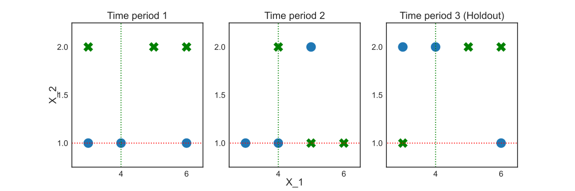
The split learned changes if we apply this algorithm to the motivational example. The TRT splits the two classes using $X_1 \leq 4$. In Figure 2, the TRT decision boundary for a single split is represented by the green dotted line, while the DT one is represented by the red dotted line.

Synthetic example

After a simple and illustrative example, we move to a synthetic data case to show a more realistic setting, including the hyper-parameter definition. Once again, we include a spurious feature in the data generating process: a variable that suffers a concept drift that makes it non-stable in the training set, $X_2$. The example is extreme, since $X_2$ mimics $Y$ in $t=1$, while it is random in $t=2$, both of them available for training. The $X_2$ keeps random in the following periods, which consist the holdout set. It emulates the hypothesis that unstable properties are less likely to persist.

where \(e\) is the time period variable, which is our environment. In the training, we have two training environments \(\epsilon_{train} = \{1, 2\}\). The \(f(e)\) defines \(X_2\) following:

We make it a binary classification task by converting $y$ to a positive class when greater than $0.5$ and to the negative one otherwise. The holdout is composed of the following periods, starting at $t=3$.

At first, we apply the TRT and the DT using similar hyper-parameters: 30 as maximum depth, 0.01 as minimum impurity decrease, 10 as a minimum sample by period for the TRT, and 20 as a minimum sample to split for the DT since we have two periods. In this case, the TRT presents an AUC of 0.83 in train and 0.81 in the holdout, while the DT performs around 0.92 AUC in training and 0.64 in the holdout. It shows how the TRT avoids learning from the spurious variable $X_2$, which lowers its training performance but makes it succeed in the holdout, while the DT goes in the opposite direction. However, we need to define the hyper-parameters following a process and objective criteria in a real-world case. In the following subsection, we show how to execute this step when using the TRT.

Hyper-parameter optimization

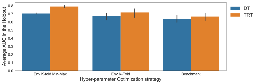
We will apply the traditional K-fold to the example as the benchmark. However, this design pools the data from the periods during the hyper-parameter selection and then select the parameters with the highest performance. This process does not favor the period-wise design from TRT. We use a K-fold that generates folds containing just one environment, used as test folds to overcome it. We identify this approach as Environment K-Folds (Env K-Folds). Similar to what we use to learn the best split in the TRT, Besides taking the average performance in the folds to decide the hyper-parameters, we evaluate a second strategy when using the Env K-Folds. First, we average the performance in all folds consisting of the same environment and hyper-parameter set. We group by only hyper-parameters sets and select the minimum performance, the worst environment case. Finally, we take the set with the highest performance among the worst cases to determine the model using the best worst case. We identify this approach as Env K-folds Min-Max.

We bootstrap the data and repeat the process ten times to evaluate these different designs. The results are the average of these ten best models following each approach. As seen in Figure 3, the TRT performs significantly better than the DT in the holdout set when using the Env K-folds Min-Max, while the other two strategies are similar.

The period-wise performance aggregation

The examples presented use the worst case from the periods to decide the best split in Equation \ref{eq:best_split}. The worst case is summarizing many periods using one, which can be undesirable under a possible problematic segment. However, one can use any aggregation function to combine the multiple periods’ performance, like the average. In this subsection, we briefly discuss this choice.

Applying the average case to the first example, the TRT and the DT would do the same split. It happens because the spurious period’s performance is so strong that it is not enough to average it with a random-performing to avoid exploiting the spurious variable. As the number of time segments increases, individual periods will have less importance in the decision. Nevertheless, the same thing happens to the DT as the volume of data increases. The difference is that the TRT is biased to care more about the persistence of the relationship than the volume of data generated under it.

The package

The TRT is available as a particular case of its ensemble form in the time-robust-forest package. To install it, simply use pip install time-robust-forest. Below there is an example of how to use it.

from time_robust_forest.models import TimeForestClassifier

features = ["x_1", "x_2"]
time_column = "periods"
target = "y"

model = TimeForestClassifier(time_column=time_column)

model.fit(training_data[features + [time_column]], training_data[target])
predictions = model.predict_proba(test_data[features])[:, 1]

To use the environment-wise optimization:

from time_robust_forest.hyper_opt import env_wise_hyper_opt

params_grid = {"n_estimators": [30, 60, 120],
              "max_depth": [5, 10],
              "min_impurity_decrease": [1e-1, 1e-3, 0],
              "min_sample_periods": [5, 10, 30],
              "period_criterion": ["max", "avg"]}

model = TimeForestClassifier(time_column=time_column)

opt_param = env_wise_hyper_opt(training_data[features + [time_column]],
                               training_data[TARGET],
                               model,
                               time_column,
                               params_grid,
                               cv=5,
                               score=roc_auc_score)

Conclusion

The TRT offers a simple way to inform environment details with a standard use case that explores time, an omnipresent characteristic of any dataset. Whenever additional domain-specific environment information is available, it can be easily integrated by concatenating the time with the new information. For example, year-hospital, month-country, month-branch, etc.

In a future post, we will apply the Time Robust Forest to real datasets and compare it to a benchmark that does not leverage the time information.