Index

1. Introduction
2. Pearson tying spurious correlation to causation
3. Spuriousness as a transient state, a nonsense relationship
4. Reichenbach’s common cause principle
5. Pearl, a precise causal interpretation and a general framework to spot spuriousness
6. How does it impact Machine Learning?
7. Environments
8. Causal relationships can still suffer from bias
9. How does concept drift fit?
10. Conclusion

    Introduction

When we look to the definition of spurious correlation as something not genuine or counterfeit, and the way we informally use it in the data science community, it sounds pretty right. Still, when we put the many contexts in which we apply this term, its definition becomes a blur, making the whole discussion of the different challenges under the “spuriousness” term difficult.

In the “Why should I trust you?” by Ribeiro (2016) ¹, model inputs that introduce spurious correlations are contrasted with features that are informative in the real world. Then the Wolf Vs. The husky classifier example is presented and, though it’s not directly said, the snow is considered a spurious correlation, which is also called “undesired correlation” in the article.

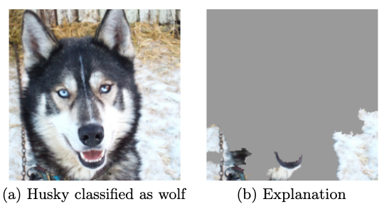
In this example, we classify it as a flawed model due to mainly or exclusively using the “snow” to split the classes. So here, we tie the spurious correlation definition to a specific task, model, dataset, or even a combination of them. In this direction, spuriousness becomes a relative concept instead of an absolute definition of two variables.

As Léon Bottou says in the “Learning Representations Using Causal Invariance” presentation, though it’s a flawed model, it’s statistically correct in this static image dataset. And that’s the problem: it’s working as intended, but it’s wrong.

Let’s take a look at another spurious correlation case.

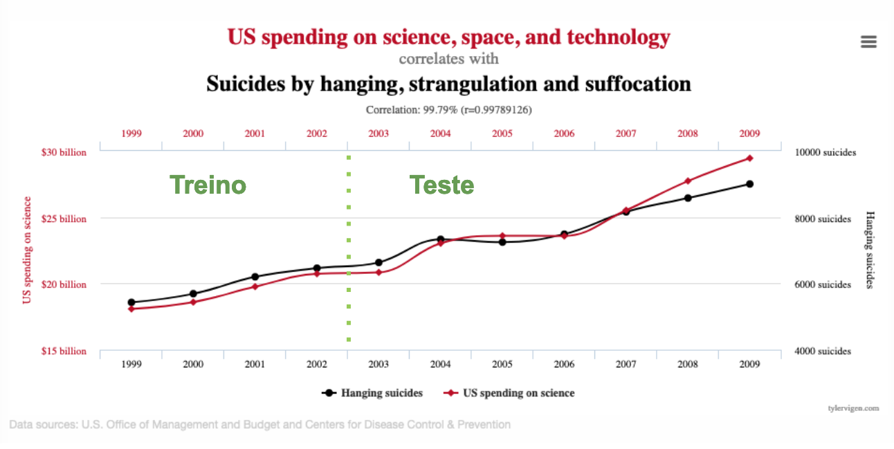
We all end up at some point laughing about the correlations presented by the famous collection in “Spurious correlation” ². We feel confident as something so ridiculous would never fool our validation strategy. But what if we have the following split?

Still! We would certainly say it’s nonsense, temporary, and an extreme coincidence. Well, it’s easy to spot it in a two-variable scenario, but it might become problematic as the number of variables involved grow.

One last example to illustrate the discussion: I’ve organized a dataset containing news about Brazilian soccer clubs from 2015, updating it monthly.

In an NLP task to identify the club subject the author is talking about using the words contained on it, we’ll find many cases like the one below: a player can transfer to a new club and change how his name is associated with it. Is the feature about this player spurious?

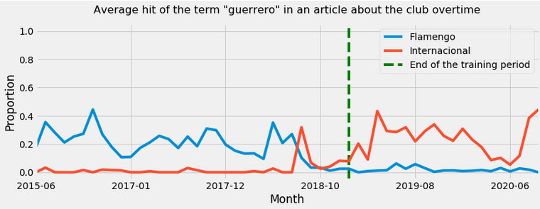
Here the correlation is certainly not an accident, but it’s transient. It’s clear a specific club is not defined by a particular player: they come and go; we still recognize it as the same club.

Let’s go through previous discussions and definitions about spurious correlation to better grasp spuriousness and manage these cases.

Pearson tying spurious correlation to causation

For someone known for the “Pearson correlation”, funnily, Pearson ³ starts from a causation definition before he states the importance of this broader association type called correlation, which ranges from absolute independence to complete dependence.

If the unit A be always preceded, accompanied or followed by B, and without A, B does not take place, then we are accustomed to speak of a causal relationship between A and B

– Pearson ⁴

Then, having the notions of causation and correlation, Pearson defines the spurious correlation.

Causation is correlation, except when correlation is spurious, when correlation is not causation.

– Pearson ³

So from everything that’s associated, it’s a spurious association when it’s not via a causal relationship. For Pearson, correlation is powerful because, though it’s not always causation, sometimes it is! It equips people with the power of estimating this association factor.

Spuriousness as a transient state, a nonsense relationship

Yule (1926) ⁵ presents the kind of relationship we consider funny and nonsense.

… But what one feels about such a correlation is, not that it must be interpreted in terms of some very indirect catena of causation, but that is has no meaning at all; that in non-technical terms it is simply a fluke, and if we had or could have experience of the two variables over a much longer period of time we could not find any appreciable correlation between them.

– Yule ⁵

The fact it’s nonsense makes us associate it with a transient relationship - otherwise, a persistent “strange correlation” would push humanity to research it until it’s not nonsense.

The Husky and club news examples don’t seem to fit here. While the correlation between US spending on science and Suicides does fit.

Yule (1926) characterizes this case as a result of undersized samples in a shorter period than needed to determine the actual correlation.

Though the discussion in the article and the examples from the Spurious Correlation website are about this exact case - time series in a reasonably short time - it’s not that rare this kind of nonsense correlation happens in extensive tabular data. If we take the parallel of something that happens by chance and would probably not keep observing as time passes, some features correlate with the supervised learning target even if shuffled. This enables feature selection procedures like Permutation Importance (Pimp) ⁶.

Reichenbach’s common cause principle

Reichenbach (1956) ⁷ introduces a third variable to define causality on his common cause principle, extracted from Peters (2017) ⁸:

If two random variables \(X\) and \(Y\) are statistically dependent \((Y \not \perp \!\!\! \not \perp X)\) then exists a third variable \(Z\) that causally influences both. (As a special case, \(Z\) may coincide with either \(X\) or \(Y\).) Furthermore, this variable \(Z\) screens \(X\) and \(Y\) from each other in the sense that given \(Z\), they become independent, \(X \perp \!\!\! \perp Y\).

This third variable \(Z\), also known as a confounder when not in the particular case, now becomes a source of a spurious correlation.

A classic example of the common cause is the observed correlation between ice cream consumption (\(X\)) and crime rate (\(Y\)), which is confounded by day temperature (\(Z\)). So in the summer, when it’s hot, people consume more ice cream, but they also occupy more public spaces and are more prone to crimes.

We represent it in the following causal directed acyclic graph (DAG), a graphical representation where causes are connected to effects by an arrow.

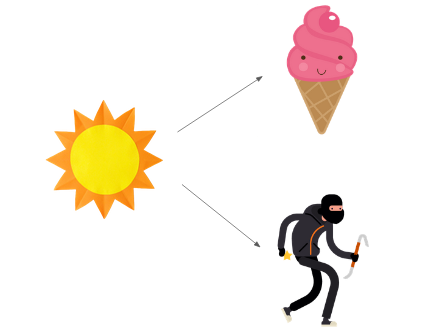
See how now it’s part of the causal structure that defines the phenomena involving \(X\), \(Y\), and \(Z\), which does not sound well with the nonsense view of spuriousness - we can come up with a bit of story to explain it. We are not talking about something we observe by chance, but \(Z\) would cause this confusion about \(X\) and \(Y\) under every circumstance.

Notice this principle does not cover other sources of non-causal association between \(X\) and \(Y\) which is not related to a common cause, but by conditioning in a common effect, which creates selection bias.

Pearl, a precise causal interpretation and a general framework to spot spuriousness

As noted by Simon (1954) ⁹, the spurious correlation problem needs a “precise and operationally meaningful definition of causality”. Reinchenbach (1956) ⁷ took it further from Pearson’s definition, then Pearl (2009) ¹⁰ introduced the context to make it more general and precise and a whole set of results and operational tools for causality.

We can define the spurious association with temporal information (the option for the temporal version is due to not being necessary to prove spuriousness in both directions):

Two variable \(X\) and \(Y\) are spuriously associated if they are dependent in some context \(S\), if \(X\) preceeds \(Y\), and if there exists a variable \(Z\) satisfying:

\[\newcommand{\indep}{\perp \!\!\! \perp} \newcommand{\dep}{\not \perp \!\!\! \not \perp}\] \[\begin{align} \begin{split} {}& (Z \indep Y \mid S) \\ {}& (Z \dep X \mid S) \\ \end{split} \end{align}\]

The context here means a set of variables at specific values, including the empty set.

We can extend from this definition that every relationship leaking from a non-causal path, known as the Backdoor path, is a spurious association. A non-causal path is every path in a causal DAG one can connect two nodes (variables) while disrespecting the arrow directions. Just as we could do connecting ice cream and robbery in the previous example.

Here it’s a persistent problem arising from the same source, but the correlation would vary.

How does it impact Machine Learning?

While the backdoor path is a curse for causal inference, it’s a glory for predictive tasks in Machine Learning. It’s usually the case we don’t have access to direct effects, so any “leakage” coming from any direction is a signal, and a model can use it to predict the most likely outcome.

But it’s a cheap glory, as endless limitations arise from this.

This behavior has numerous drawbacks, like the ones pointed in the Husky from the introduction. A similar one comes from Beery (2018) ¹¹, with cows and grass, camels and sand.

Arjovsky et al. (2019) ¹² discuss the implications in ML before offering a new framework to deal with it, which I’ll cover in a future post.

Intuitively, a correlation is spurious when we do not expect it to hold in the future in the same manner as it held in the past. In other words, spurious correlations do not appear to be stable properties.

– Arjovsky et al. ¹²

But this stability is not only in respect to the future. A dataset can be generated by different data generating processes, like the collection methodology. Imagine a healthcare dataset collected from various hospitals or in different countries. Or a computer vision dataset with pictures taken from different cameras.

This breaks one of the most critical assumptions for the Empirical Risk Minimization paradigm in supervised learning: train and test come from an i.i.d sample from the sample distribution.

the i.i.d. assumption is the great lie of machine learning.

– Zoubin Ghahramani ¹³

In a past presentation about Validation, the process to verify if a particular model generalizes, I warned about something I’ve learned from real-life applications: \(X\) is mutant!

In this same presentation, some validation methods were presented, like splitting the data between training-past and testing-future, to assess how dependent the machine learning model is on spurious relations from the specific contexts present in the past.

As Arjovsky et al. (2019) ¹² states: shuffling data is something that we do, not something Nature does.

The authors bring yet another caveat of how ML is impacted: in over-parameterized models, like Neural Networks. The procedure that we are used to training it is going to prefer the solutions with the smallest capacity, a measure of the representational power of a model. This makes these models prefer simple rules instead of complex relationships. It might be the case this simple rule is spurious, like associating the green color to recognize cows instead of a complete profile of its shape.

Notice this is one of the sources of overfitting, a situation our model has learned the idiosyncrasies of the training set and fails to generalize. It’s not the only source since it’s easy to show one can use a very complex model to learn sample by sample from a training set and fail to generalize in a test set sampled from the same distribution from the train.

Environments

To make the discussion about the relationship between machine learning and spurious correlation more interesting, we bring two other concepts into play: intervention and environment (or context).

We need to define intervention because it’s required to determine environments.

An intervention replaces one or more equations presented in a Structure Equation Model (SEM). It’s basically changing the causal relationship between the variables of our problem. A valid intervention does not destroy too much the causal connection involving \(Y\), the variable of interest we’re trying to predict.

Then the set of environments \(\epsilon_{all}\) is composed by all the possible cases generated by all possible valid interventions in an SEM as long as the interventions keep the graph acyclic, it doesn’t change \(\mathbb{E}[Y \mid Pa(Y)]\), and the variance \(V[Y \mid Pa(A)]\) if finite.

To exemplify, we use the same illustrative case from Arjovsky et at (2019) ¹²:

This is the causal graph that represents the following Structured Equation Model (SEM):

\[\begin{align} \begin{split} X_1 {}& \leftarrow \mathbb{N}(0, \sigma^2) \\ Y {}& \leftarrow X_1 + \mathbb{N}(0, \sigma^2) \\ X_2 {}& \leftarrow Y + \mathbb{N}(0, 1) \\ \end{split} \end{align}\]

The \(\sigma^2\) is the thing we can vary to represent different environments. Imagine we could have some environments in the training data (\(\epsilon_{tr} = \{\text{replace } \sigma^2 \text{ by } 10, \text{replace } \sigma^2 \text{ by } 20\}\)).

Then the authors show how the linear model built with this data can be different depending on the variables we use and the environment \(e\) when we want to predict \(\hat{Y}^{e} = X_1^e \hat{\alpha}_1 + X_2^e \hat{\alpha}_2\):

• Regress using \(X_1^e\) and obtain \(\hat{\alpha}_1 = 1\) and \(\hat{\alpha}_2 = 0\)
• Regress using \(X_2^e\) and obtain \(\hat{\alpha}_1 = 0\) and \(\hat{\alpha}_2 = \sigma(e)/(\sigma(e) + \frac{1}{2})\)
• Regress using \(X_1^e\) and obtain \(\hat{\alpha}_1 = 1/(\sigma(e) + 1)\) and \(\hat{\alpha}_2 = \sigma(e)/(\sigma(e) + 1)\)

See how only the first case gives us an invariant estimator since the other two options depend on \(e\). And that’s how spurious correlations related to idiosyncrasies from the environments available in training will affect the genuine relationship and make this model likely low-performing for unseen environments, which we all expect to encounter when deploying a model in real life.

Notice your model would do a pretty good job in a traditional validation schema. If you pool together all the data, shuffle, get a random sample to train and another to test, train, and validate, you wouldn’t be surprised by anything. Your model would be using the specific correlations present in the training environments to do good in other samples from these same training environments. However, this won’t be the case in production. And it would be better to have learned the invariant estimator from case 1, even if it means a higher test set error because it’s the best model to face a real-world scenario where the environment changes.

Here we can see how the transient notion of spuriousness is contrasted with the invariance notion for causal.

Causal relationships can still suffer from bias

Even if we rely on the mechanism \(P( Y \mid X_1)\), there are ways a causal relationship can be infected. Introducing causal relationships into ML makes us take advantage of them, but it also brings all of its challenges, like hidden confounding and lack of identifiability.

Let’s use a slightly modified example from the previous causal graph and make the environment explicit as defining \(X_1\) and \(X_2\).

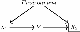
Someone or some process could filter examples based on the \(X_2\) value, which opens a non-causal path between \(X_1\) and \(Y\). By doing so, even if you use only \(X_1\) to estimate your model, it won’t retrieve the invariant estimator. Even if we are able to control by the Environment, the selection bias might have compromised the positivity (\(P(X_1 \mid \text{Environment}) > 0\)) and make it impossible to estimate the real relationship between \(X_1\) and \(Y\).

How does concept drift fit?

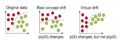
There are many things under the dataset shift or concept drift definition. Here we’ll expose only two concepts, the virtual concept drift and the real concept drift.

• Virtual concept drift: \(P(X)\) changes;
• Real concept drift: \(P(y \mid X)\) changes;

Basically, in the virtual, the input distribution change. In the real, a mechanism, the way we map inputs to outputs, changes. These concepts are illustrated by Kadam (2019) ¹⁴:

When the virtual concept drift happens, there’s little to worry about. You might want to review the policy you have built on top of the model since the distribution of input cases has changed, and the previous decision-making process can imply different things. Your model aggregated metric is different in a sample with an eclectic mix of examples.

There’s nothing causal or anti-causal in the inputs’ distribution.

When we are estimating \(\hat{Y}\), we’re interested in its mechanism. In the examples above, we saw the mechanism of interest was \(P(Y \mid X_1)\). So even if a real concept drift happens to \(P(X_2 \mid Y)\), it shouldn’t be a problem if we have learned the invariant predictor. So here’s another downside of using spurious correlations: it exposes you to changes in components you shouldn’t even be using.

We don’t let intervention be made in the variable of interest (\(Y\)) to be considered a new environment. In this case, it’s a sole concept drift problem, and the model needs to be retrained to learn the new concept.

After all the definitions, we can get back to the third example from the introduction, about players and clubs. It’s the trickiest. It might be the case we shouldn’t expect the term \(P( Club \mid \text{Specific Player})\) to be invariant because it’s not a causal mechanism when we draw the DAG for this specific case. Even if it’s the case, there’s a chance a “social phenomena” suffers more of real concept drift, and it’s far from the invariance expected for physical laws. We might be obligated to do a trade-off between including more causal terms prone to real concept drift to have a better performance in the short term. For example, the series of interventions that define the following environments might first change the relationship with player A and Club X, then with player B, and so on.

Conclusion

We talked a lot about causality, prediction problems from Machine Learning, environments, and concept drift to describe spurious correlation.

One very special property was identified: Invariance, which is really cool and deserves a particular discussion.

It should be clear spurious correlations are a way more harmful problem than the cheerful examples we use to illustrate it suggest, which always sound far from the day-to-day application.

Since causality is tied to spuriousness, part of Machine Learning development seems to go through it.

---

		
		  @article{moneda2021spurious-correlation-blogpost,
		  author = {Moneda, Luis},
		  title = Spurious correlation, machine learning, and causality,
		  journal = {Blogpost at lgmoneda.github.io},
		  year = {2021},
		  howpublished = {\url{lgmoneda.github.io}},
		  }