Index

1. Introduction
2. The principle of independent mechanisms
3. Real data example
4. Environments and invariance
5. Why is it important to get the causal relationship right if I’m not doing causal inference?
6. Conclusion
7. References

Introduction

This post aims to introduce the concept of Independent causal mechanisms and invariance. It’s an essential principle of causal inference. Still, it’s also related to the many drawbacks of traditional Machine Learning, described in the previous post “Spurious correlation, machine learning, and causality”, which I recommend reading before this one.

The principle of independent mechanisms

The primary example to illustrate this principle is the altitude and temperature relationship. It can be found on Peters (2017) ¹.

Imagine we have a dataset with the altitude and the average annual temperature from different cities in a country. So we have the joint probability \(p(a, t)\).

One can decompose this probability in two different ways.

These two factorizations imply different causal structures. The first represents the causal graph \(T \rightarrow A\), while the second is \(A \rightarrow T\). How would we know what the right direction is?

Before we even talk about the implications of these two possibilities, we can imagine interventions on this problem - even if they are not reasonable or feasible.

Intervention 1: we somehow elevate all the cities in our dataset. What is the effect on the average annual temperature? Well, considering what we know about physics, it’s going to drop.

Intervention 2: we artificially change the city’s temperature using a giant air conditioner. What is the effect on altitude? We wouldn’t expect any change.

This little imagination exercise reveals an intervention that could help us disambiguate such a situation. We intervene in the hypothesized cause, and we watch for the effect. Though someone can estimate from data both relationships - see, nothing holds you to regress \(T\) on \(A\) or \(A\) on \(T\) - one of them is going to be a simple association, while the other reveals a causation mechanism in which one can convert changes in \(A\) into changes in \(T\).

What if the intervention is not available and our intuition can’t help us?

Instead of thinking about this data coming from a single country, let’s now imagine we have different datasets coming from two countries, and we’re going to identify them by a superscript.

Brazil and Germany have a different distribution of cities’ altitude, but shouldn’t the relationship between altitude and temperature be equal no matter where we measure it?

It’s indeed what happens (in idealized settings), but only when we get the causal direction right.

So we could rewrite it as:

This invariance under different countries would enable Transfer Learning. Since it’s unnecessary to learn from German data to predict how to translate its cities’ altitude into temperature predictions, we can reuse the same module learned for other countries.

Real data example

Identifying the relationships and their directions is a task known as causal structure discovery, causal discovery, or structure identification. And this is what we want here: decide between \(T \rightarrow A\) and \(A \rightarrow T\).

With the assumption the function connecting \(A\) and \(T\) is an Additive Noise Model (ANM), there’s a method based on the independence of residuals.

The assumption is needed to explore the property that arises of having a “right” direction (from cause to effect). Assuming an Additive Noise Model:

Where \(Y\) and the noise \(N\) are independent. Then there’s no such model that:

And \(X\) is independent of \(N\).

Then, the method to verify:

1. Fit a function \(f\) as a non-linear model of \(X\) on \(Y\)
2. Compute the residual \(N = Y - f(X)\)
3. Check whether \(N\) and \(X\) are statistically independent

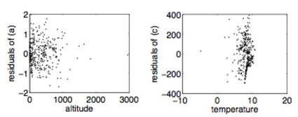
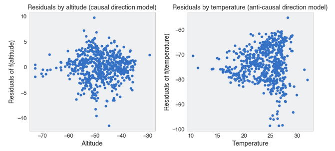
The results from Mooji (2016) ², who also provides evidence of this method for other real data cases, show a strong dependency on the anti-causal direction. In the horizontal axis of the two plots, we have the \(X\) variable, which is the input, the cause. We can see that when the temperature is taken as the cause of altitude (second plot), we observe the dependency.

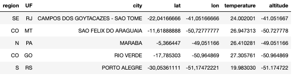
Let’s try to reproduce it with different data! So we need altitude and temperature. We’re going to use data from Brazil. The raw data comes from Inmet. It was required to process all the files, get the average temperature for the year (2020), exclude instances without data, and get rid of one possibly wrong data point. You can find the final data here.

We have the following dataframe:

Then we just follow the method in a few lines of code.

from lightgbm import LGBMRegressor

### Causal model
alt_temp_model = LGBMRegressor()
alt_temp_model.fit(df["altitude"].values.reshape(-1, 1), df["temperature"].values)
predicted_temperature = alt_temp_model.predict(df["altitude"].values.reshape(-1, 1))
alt_temp_residuals = df["temperature"].values - predicted_temperature

### Anti-causal model
temp_alt_model = LGBMRegressor()
temp_alt_model.fit(df["temperature"].values.reshape(-1, 1), df["altitude"].values)
predicted_altitude = alt_temp_model.predict(df["temperature"].values.reshape(-1, 1))
temp_alt_residuals = df["altitude"].values - predicted_altitude

The result is pretty much the same. If you estimate the Pearson correlation between the residuals and the input, you get a 0.077 (p-value, 0.06) for the anti-causal direction and 0.004 (p-value, 0.92) for the causal order.

Environments and invariance

For the needed definitions, see the section “Environments” from the previous post Spurious correlation, machine learning, and causality. Here we discuss its notion at a high level to elucidate the examples.

If there’s no path between mechanisms, they are expected to be invariant under interventions in the other mechanisms underplay and changes in the exogenous variables, which are mechanisms that are not being considered. Still, they play a role in the phenomena like precipitation that could impact temperature in the \(Altitude \rightarrow Temperature\) example.

Since intervention in a particular mechanism doesn’t affect the others, different environments share common pieces of causal knowledge. And this is not only interesting because we can transfer learning, but it then becomes a constraint for learning in the first place.

And environments can assume different forms: different countries, policies, time, companies, hospitals. If there’s no confounding, the conditional probability \(P( Y \mid Pa(Y))\) should be the same across the different environments in the dataset.

This is very interesting because while this kind of environmental change is seen as the machine learning practitioner’s nightmare, it might be precisely our redemption.

The Spurious correlation post post contains Arjovsky (2019) ³ demonstration on how the genuine causal relationship stands in every environment. Moving from the causal discovery example with two variables where we want to find the right direction, let’s explore the case of having a target \(Y\) and two input variables, \(X_1\) and \(X_2\).

Let’s create two environments and define the data generation process as follow:

import pandas as pd
import numpy as np

from sklearn.linear_model import LinearRegression


POPULATION = 10000
environments = [0.1, 1]
data = pd.DataFrame()
data["environment"] = np.concatenate(
                 [int(POPULATION/2) * [environment] for environment in environments],
                 axis=0)

data["x_1"] = data.apply(lambda x: np.random.normal(0, x["environment"]), axis=1)
data["y"] = data.apply(lambda x: 1 * x["x_1"] + np.random.normal(0, 1), axis=1)
data["x_2"] = data.apply(lambda x: x["y"] * x["environment"] + np.random.normal(0, 1), axis=1)

Let’s start by pooling the data from both environments and estimating \(Y\) trying three different specifications: \(X_1\), \(X_2\) and \((X_1, X_2)\)

LinearRegression(fit_intercept=False).fit(data["x_1"].values.reshape(-1, 1), data["y"]).coef_
>>> 1.01708804

LinearRegression(fit_intercept=False).fit(data["x_2"].values.reshape(-1, 1), data["y"]).coef_
>>> 0.52581294

LinearRegression(fit_intercept=False).fit(data[["x_1", "x_2"]], data["y"]).coef_
>>> [0.65424076, 0.36760065]

We only get the true parameter for the data generating process when we regress \(Y\) only on \(X_1\).

Now let’s see how it looks when we split the data into the two environments.

data.groupby("environment").apply(lambda x: LinearRegression(fit_intercept=False)
                             .fit(x["x_1"].values.reshape(-1, 1), x["y"]).coef_)


>>>   environment
>>>   0.1    [1.0716022375046923]
>>>   1.0    [1.0164936578119834]

data.groupby("environment").apply(lambda x: LinearRegression(fit_intercept=False)
                             .fit(x["x_2"].values.reshape(-1, 1), x["y"]).coef_)

>>>   environment
>>>   0.1    [0.10892565273942922]
>>>   1.0     [0.6681684820400771]

data.groupby("environment").apply(lambda x: LinearRegression(fit_intercept=False)
                             .fit(x[["x_1", "x_2"]].values, x["y"]).coef_)

>>>   environment
>>>   0.1    [1.0379742976008124, 0.10549085567094083]
>>>   1.0     [0.5188938784812798, 0.5004242700296184]

Notice the only case where the parameter is the same in both environments is when we use only the causal variables to predict the output. In the other cases, the parameters change when estimated using only data from a particular environment.

What if we invert the direction and use \(X_1\) as the output and \(Y\) as input?

data.groupby("environment").apply(lambda x: LinearRegression(fit_intercept=False)
                             .fit(x["y"].values.reshape(-1, 1), x["x_1"]).coef_)

>>>   environment
>>>   0.1    [0.011438451217063788]
>>>   1.0      [0.4871463714326833]

The importance of this property is also highlighted in Goyal (2020) ⁴. When talking about important Inductive bias for Machine Learning, “stable properties of the world” and “reusable knowledge pieces” are related to independent causal mechanisms. For the learning part, it’s noted how we can explore the interventions and changes in environments to learn from it since it reveals what is invariant, non-stationary, and spurious. It brings examples of models exploring this property by Goyal (2019) ⁵ and Bengio (2019) ⁶.

Why is it important to get the causal relationship right if I’m not making causal inferences?

As we have seen, when the causal direction is correct, we could learn an independent and modular piece of knowledge called mechanism, which we can apply under different conditions to transform causes into effects.

So when things like Covariate shift happen, it becomes just a matter of a different input distribution to our invariant mechanism. But, if we have learned the anti-causal conditional probability, let’s say \(P(Cause \mid Effect)\), then a covariate shift (\(P(Effect)\) change) is going to also change the supposedly invariant mechanism.

And a covariate shift is something ubiquitous in real-world applications.

It doesn’t mean though all causal mechanisms are fixed. They still can be non-stationary, depending on the application. Our notion of physics agrees with stationary rules for the universe, but we could have causal relationships like years of work experience and wage. When the conditional probability changes, then it’s a concept drift. Though there’s little to do in this case, we’re surely in a better place if we have learned the right causal conditional probability than the anti-causal.

Conclusion

The Principle of Independent Mechanism offers a set of intuitive assumptions we can find evidence in actual cases. Suppose there’s such robust decomposition of joint probabilities into independent mechanisms that would be invariant to environment changes, interventions, and previous policies. In that case, it becomes then attractive to explore such benefits in Machine Learning models, whose generalization power suffers under environment changes and dataset shifts. We’ll see how this principle is leveraged in Machine Learning in the following posts.

References