Index
Introduction
This is the second post of the series “Exploring invariance in Machine Learning”, I recommend reading the first post about Invariant Causal Prediction, and the ones about spuriousness and the independent causal mechanism principle.
Environment
Since the Environment concept is so important for the framework, we present the definition from Arjovsky (2019) 1:
Definition: Consider an SCM defining how the random variables \((X_1, ..., X_d, Y)\) define each other, and the goal of learning a predictive model for \(Y\) using \(X\), then the set of environments \(\epsilon_{all}\) is defined by the distributions \(P(Y^e, X^e)\) generated by a valid intervention \(e\). An intervention \(e \in \epsilon_{all}\) is valid if the causal graph derived from the SCM stills acyclic, the variable of interest \(Y\) expectation persists, \(\mathbb{E}[Y^e \mid Pa(Y)] = \mathbb{E}[Y \mid Pa(Y)]\), and the variance \(V[Y^e \mid Pa(Y)]\) remains finite.
Intuitively, an environment can be the different devices used to capture the images in a computer vision problem; the hospitals from which we collected the data about patients; countries; backgrounds of images. It’s a set of conditions that can be interpreted as the background “context” of them problem. It can be generated by an intentional, unknown, or not controlled intervention.
Arjovsky (2019) use as example the background when classifying Camels and Cows, and how it is easy for a model to become a sand and grass classifier instead, which means exploring a spurious correlation to succeed.
Invariant Risk Minimization
In the Invariant Risk Minimization framework, the preference for invariance through the environments is expressed in the loss function by an additional term and an iteration on all the environments in the training set1.
The Out of Distribution (OOD) Risk is defined as:
\begin{equation} \label{eq:8} R^{OOD}(f) = \min_{e \in \varepsilon_{all}}R^{e}(f) \end{equation}
The subscript all means we want to minimize it for all possible contexts and not only the ones in the training data.
The risk under a certain environment \(e\) is defined as \(R^{e}(f) := \mathbb{E}_{X^{e}, Y^{e}}[l(f(X^{e}, Y^{e}))]\), where \(l\) is any loss function.
However, the function \(f\) will be decomposed into two stages. The first stage transforms the data from the different contexts to find a representation that enables a single optimal classifier for all of them. The second searches for this optimal classifier.
Definition: A data representation \(\Phi: \mathcal{X} \rightarrow \mathcal{H}\) elicits an invariant predictor \(\omega \circ \Phi\) on all the contexts \(\varepsilon\) if there’s a model \(\omega: \mathcal{H} \rightarrow \mathcal{Y}\) optimal for all contexts at the same time, it is, \(\omega \in arg\min_{\bar{\omega}: \mathcal{H} \rightarrow \mathcal{Y}} R^{e}(\bar{\omega} \circ \Phi)\) for all \(e \in \varepsilon\).
\(\mathcal{H}\) is the latent space in which the algorithm searches a representation that enables the existence of the model \(\omega\). Therefore, the IRM paradigm can be described by the following optimization.
\[\begin{equation} \label{eq:9} \begin{split} \min_{\substack{\Phi: \mathcal{X} \rightarrow \mathcal{H} \\ \omega:\mathcal{H} \rightarrow \mathcal{Y}}} \text{ } {}& \sum_{e \in \varepsilon_{train}}R^{e}( \omega \circ \Phi) \\ {}& \text{strict to } \omega \in arg\min_{\bar{\omega} \mathcal{H} \rightarrow \mathcal{Y}} R^{e}(\bar{\omega} \circ \Phi), \text{ for all } e \in \varepsilon \end{split} \end{equation}\]However, this optimization is hard to solve since it involves \(\omega\) and \(\Phi\) at the same time. To work around this problem, the authors propose the following version:
\begin{equation} \label{eq:10} \begin{split} \min_{\substack{\Phi: \mathcal{X} \rightarrow \mathcal{H}}} \text{ } {}& \sum_{e \in \varepsilon_{train}}R^{e}(\Phi) + \lambda \Vert {\nabla_{\omega \mid \omega = 1.0}R^{e}(\omega \circ \Phi)}\Vert^{2} \end{split} \end{equation}
Where \(\Phi\) become the complete invariant predictor without the need of composing it with \(\omega\), which is fixed as \(1\), turning into a dummy model. The gradient norm penalty in the loss function, the second term in \(R\), is used to measure how optimal the model is in every context \(e\). \(\lambda \in [0, \infty ]\) is the regularizer term that balances between the predictive power, the one minimizing \(R\) following the ERM paradigm, and the invariance of the predictor \(1 . \Phi(x)\).
Thus the objective function can be expressed as:
\begin{equation} \label{eq:11} L_{IRM}(\Phi, \omega) = \sum_{e \in \varepsilon_{tr}} R^{e}(\omega \circ \Phi) + \lambda \mathbb{D}(\omega, \Phi, e) \end{equation}
The \(\mathbb{D}\) represents the penalization and we need it to be differentiable in respect to \(\Phi\) and \(\omega\).
In the case of learning an invariant predictor \(\omega \circ \Phi\), where \(\omega\) is a linear regression learned with least squares, we would have the penalty \(\mathbb{D}_{lin}\).
\[\mathbb{D}_{lin}(\omega, \Phi, e) = \Vert{\mathbb{E}_{X^{e}}[\Phi(X^{e}) \Phi(X^{e})^{T}]\omega - \mathbb{E}_{X^{e}, Y^{e}}[\Phi(X^{e})Y^{e}]}\Vert^{2}\]It is a differentiable function that enable us to optimize the objective function using gradient descent.
The conditions about what can be considered an environment in \(\varepsilon_{all}\) follows the definition from the previous section. They need to be respect in order to be able to train with \(\varepsilon_{train}\) and have OOD, which implies optimal performance in all the possible valid environments.
As seen, an environment can be seen as an intervention, which is when we modify one or more equations from a SEM, forcing particular values or functional forms, which is interesting to observe how this intervention will impact the other quantities involved in the same SCM.
Consider the SEM \(\mathcal{C} = (\mathcal{S}, \mathcal{N})\). An intervention \(e\) in \(\mathcal{C}\) is the replacement of one or more equations to obtain a new SEM, \(\mathcal{C}^{e} = (\mathcal{S}^{e}, \mathcal{N}^{e})\), represented by:
\[\begin{equation} \mathcal{S}_{I}^{E} : X^{e}_{i} \rightarrow f^{e}_{i}(Pa^{e}(X^{e}_{i}), N^{e}_{i}) \end{equation}\]We consider the variable \(X^{e}\) was intervened if \(\mathcal{S}_{e} \neq S_{i}^{e}\), different equations, or \(N_{i} \neq N^{e}_{i}\), the noise term is different. In following example, an intervention would be changing \(X^{e}_{2}\) by \(X^{e}_{2} \rightarrow 0\), for example.
Arjovsky (2019) 1 details how the low error on \(\varepsilon_{train}\) and the invariance on \(\varepsilon_{all}\) leads to low error on \(\varepsilon_{all}\), and how learning these invariances from \(\varepsilon_{train}\) would be able to identify the same invariances we expect to see on \(\varepsilon_{all}\).
In order to learn useful invariances, it’s needed that a certain order of diversity exists in the available contexts. Two random samples from the same dataset wouldn’t be able to offer this diversity.
Deriving the IRM for the linear regression case
In order to get a deeper understanding about the steps involved in the IRM paradigm, we derive the case for the linear regression. Consider a linear regression, where \(X\) is the set of input variables, \(y\) is the target variable, \(\beta\) is the parameter vector, we want to estimate: \(\hat{y} = \hat{\beta}X\). In this case, the function \(\Phi\) takes the form of \(\beta X\).
To achieve it, we want to minimize the loss function \(L(\beta)\). Using Gradient Descent, the search for the \(\beta\)s that minimize this function happens by the successive updates on them that take the following form:
\[\begin{equation} \hat{\beta}_{t+1} = \hat{\beta}_{t} - \gamma \nabla_{\beta \mid \beta = \hat{\beta_{t}}} L(\beta) \end{equation}\]Starting in the regular case, when we use the ERM, the minimized loss function \(L\) is the mean squared error. Thus, we learn \(\hat{\beta}\) using:
\[\begin{equation} \label{eq:14} \begin{split} L(\beta) = {}& MSE = \frac{1}{n} (\hat{y} - y)(\hat{y} - y)^{T}, \text{where } \hat{y} = X \hat{\beta} \\ % \hat{\beta}_{t+1} = {}& \hat{\beta}_{t} - \gamma * \nabla f(X) \\ \nabla_{\beta \mid \beta = \hat{\beta_{t}}} L(\beta) = {}& -\frac{1}{N} X^{T}(X\hat{\beta} - y) \end{split} \end{equation}\]In the IRM, the loss function \(L_{IRM}(\Phi, \omega)\) in the objective function is composed by two parts. The first is identical to the ERM case, however, now we iterate over the set of environments available in the training set \(\varepsilon_{train}\). We distinguish the input matrix under a certain environment \(e\) as \(X^{e}\) and the target variable as \(y^{e}\). Notice that by using \(\omega = 1.0\), we obtain \(\omega \circ \Phi\) equal to \(\beta\).
\begin{equation} \label{eq:15} R^{e}(\omega \circ \Phi) = R^{e}(\hat{\beta}) = \frac{1}{n} (X^{e} \hat{\beta} - y^{e})(X^{e} \hat{\beta} - y^{e})^{T} \end{equation}
The second part of \(L_{IRM}(\Phi, \omega)\) is composed by \(\lambda\), a constant acting as a hyper-parameter, and the penalization function \(\mathbb{D}\), in this linear case it is \(\mathbb{D}_{lin}\) \ref{eq:12}. We highlight that \(\Phi\) becomes our predictor, which in this case means it is expressed by the parameters in \(\beta\).
\[\mathbb{D}_{lin}(\omega, \Phi, e) = \Vert{\mathbb{E}_{X^{e}}[(X^{e}\hat{\beta})^{T}(X^{e}\hat{\beta})]\omega - \mathbb{E}_{X^{e}, Y^{e}}[(X^{e}\hat{\beta})^{T}Y^{e}]}\Vert^{2}\]Nonetheless, to update the parameters in \(\hat{\beta}\) we need the gradient. Since \(L_{IRM}\) is composed by a sum, the gradient first term coincides with the derivation done for the ERM case, while the second term becomes \(\nabla_{w \mid w=1.0}\mathbb{D}_{lin}(\omega, \Phi, e)\). Differentiating the previous equation in respect to \(\omega\) and then replacing it by \(1.0\):
\[\begin{split} \nabla_{w \mid w=1.0}\mathbb{D}_{lin}(\omega, \Phi, e) = {}& 4 \frac{1}{N} (((X^{e} \hat{\beta})^{T} X^{e} \hat{\beta}) - ((X^{e} \hat{\beta})^{T} y)) \\ {}& (X^{e} (X^{e} \hat{\beta})^{T} - ((X^{e} \hat{\beta})^{T}y^{e})) \end{split}\]Finally, the update of the weights under the IRM paradigm is:
\[\begin{split} \hat{\beta}_{t+1} = \hat{\beta}_{t} - \gamma \sum_{e \in \varepsilon_{tr}} {}& \left[ ( -\frac{1}{N} (X^{e})^{T}(X^{e}\hat{\beta} - y^{e})) \right. \\ + {}& \lambda (4 \frac{1}{N} (((X^{e} \hat{\beta})^{T} X^{e} \hat{\beta}) - ((X^{e} \hat{\beta})^{T} y^{e})) (X^{e} (X^{e} \hat{\beta})^{T} \\ - {}& \left. ((X^{e} \hat{\beta})^{T}y^{e}))) \right] \end{split}\]Synthetic example
To exemplify, we use the equations derived in the previous section to compare the IRM to the ERM paradigm. The code is available in a github repository. Consider the following equations from the example provided by Arjovsky (2019) 1
\[\begin{split} x_{1} \sim {}& \mathbb{N}(0, \text{environment}) \\ y \sim {}& x_{1} + \mathbb{N}(0, \text{environment}) \\ x_{2} \sim {}& y + \mathbb{N}(0, 1) \\ \end{split}\]They represent our training set. The \(Environment\), however, can assume different values during the training and after it. We use \(\epsilon_{unseen}\) to represent unseen environments considering the training examples available, they would be observed only when the model is applied to new data, which is different than random examples extracted from the training set in order to validate the model.
\[\begin{split} \epsilon_{train} = {}& (0.1, 1.0) \\ \epsilon_{unseen} = {}& (0.2, 0.05, 0.5, 1.2) \\ \end{split}\]As a consequence of the environment change, the relationship between \(x_{2}\) and \(y\) will also change on its functional form, since it’s a non-causal relationship.
\[\begin{split} x_{2} \sim {}& \mathbb{N}(0, 1) \\ \end{split}\]In this scenario, we want to build a model that can be trained on the data generated by the SCM that does not overfit to the non-causal relationships present on it, in a way that when it faces a new environment during the application stage, which follows the causal relationships present in the training, but presents different spurious correlations, it is able to present a good performance.
For this illustrative example, we will use three models:
- ERM: a linear regression using gradient descent without any kind of regularization. It’s the benchmark model.
- Oracle: It’s a model built using the real parameters from the generating process for the target, and zero for any variable that doesn’t define it. In this case, \(\beta_{1} = 1\) e \(\beta_{2} = 0\).
- IRM: It uses the loss function from IRM and a lambda value optimized using only training data. It’s the challenger model. \end{itemize}
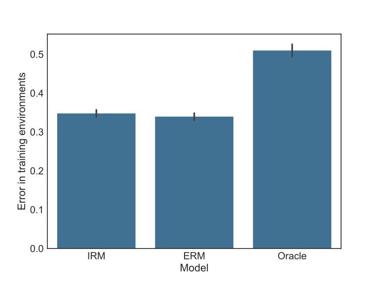
As a performance metric, we use mean squared error (MSE) to compare the models. The error is always taken from out of train data: in the first case, the test data, they come from seen environments, but it is a random sample not used for training, while in the second case, the holdout data, they come from unseen environments.
As expected, the benchmark model explores the non-causal relationships to optimize the predictive performance showing the lowest error in the test data as seen in the figure below. In this same test set, the Oracle model presents the highest error precisely by the fact it does not explore the spurious correlations from it. The challenger model is worse than the benchmark. Notice this situation is exactly the model validation framework extensively used to gather evidence about generalization power.
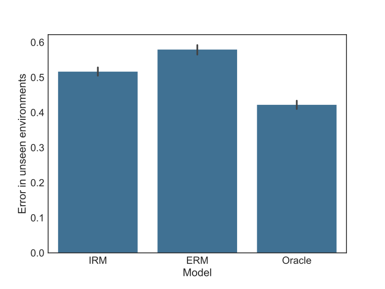
However, the context not seen in the train present different spurious correlations than the ones observed before, thus it is impossible to explore them. In this case, the performance ordering is reversed, as seen in the next figure. Now the challenger model is better than the benchmark, while both are worse than the Oracle, which is expected.
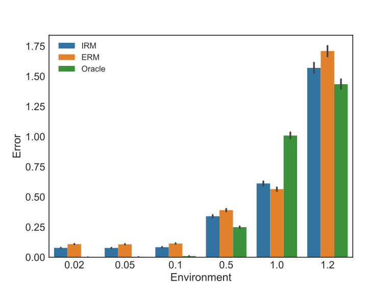
Looking to the same results in a different perspective by grouping the data by environment, we can see in the figure below how the same ordering in the aggregated results is observed in all training environments and all unseen ones.
The hypothesis to argue that IRM is a better approach to general Machine Learning problems is that it is expected in most problems to face many interventions and environments after the learning stage.
Conclusion
The IRM internalizes in the objective function from the learning algorithm our desire to rely on causal relationships to do predictions. Though we have exposed the linear case, Lu (2021) 2 brings the nonlinear version of it. This framework has received a reasonable attention from the community and it’s expected it’s going to influence new frameworks, inductive bias and designs that explores invariance.
References
Camel picture from the social share by Wolfgang Hasselmann.