Index

1. Introduction
2. Invariant Causal Prediction
3. How do I use it?
4. Synthetic example
5. What about confounding?
6. Conclusion
7. References

Introduction

As seen in the previous post Spurious correlation, machine learning, and causality, Machine Learning models face problems even when we want them to solve purely predictive tasks.

In a series of three posts, we will see how to leverage the concept of causal invariance in Machine Learning to overcome some of these problems. If you are not used to it, I recommend reading the Independent Causal Mechanisms: an introduction about the importance of invariance in Machine Learning before.

Invariant Causal Prediction

Peters (2015) ¹ explores the invariance in causal relationships through different environments to make predictive models more robust. Remember from previous posts that an environment might be interpreted as a different location, time, policy, etc. For example, healthcare data from different hospitals. Every hospital could be an environment.

Let identify the environments as \(e \in \varepsilon\) and use the linear model case. Then we have:

The superscript \(e\) is because we have a model for every environment. Where \(\mu\) is the constant intercept, \(X^{e}\) are the input variables, \(Y^{e}\) is the output, the target variable, and \(\epsilon^{e}\) is the error term.

In a supervised problem, we have a bunch of inputs, which we can also call predictors. Be \(S^*\) the set of causal predictors, which are represented by the non-zero parameters of the vector \(\gamma^*\), it is, \(S^{*} := \{k; \gamma^{*}_{k} \neq 0\}\). So \(S^*\) contains only the causal predictors, which are followed by non-zero parameters. We are interested in this subset because of all the problems presented previously about using non-causal predictors.

Hypothesis (invariant prediction): there’s a coefficient vector \(\gamma^{*} = (\gamma_{1}^{*}, ..., \gamma_{p}^{*})^{t}\)

where \(\mu \in \mathbb{R}\) is an intercept, \(\epsilon^{e}\) is a random noise with zero mean, finite variance and the same distribution \(F_{\epsilon}\) for all \(e \in \varepsilon\).

Peters (2015) ¹ shows that the parent variables of \(Y\) in a Structural Equation Model satisfy the presented hypothesis.

Two methods are presented, but we will go through only method II. First, let us simplify it.

1. For all possible subsets of input variables, do:
   1. Train a model using all contexts and only the specific input features in that subset. Calculate the residuals.
   2. Test for every context if their residuals have equal mean and variance. Combine the tests to take a single decision about rejecting this subset of features or not.
2. Find the features present in all the not rejected subsets and use them as the causal predictors.

Now that we have a high-level understanding of the process, we can formalize it:

1. For every \(S \subseteq \{1, ..., p\}\) and \(e \in \varepsilon\):
   1. Fit a linear regression with the pooled dataset, it is, from all the environments. In the case of linear regression, we get all the estimated parameters from the set \(S\), \(\hat{\beta}^{pred}(S)\). Calculate the residuals \(R = Y - X\hat{\beta}^{pred}(S)\)
   2. Test the null hypothesis that the mean from the \(R\) is equal for every environment \(I_{e}\), \(e \in \varepsilon\), using a two sample t test for the residuals in \(I_e\) and the ones in \(I_{-e}\) (all the environments, except for \(e\)), and combine the test to all the contexts \(e \in \varepsilon\) using the Bonferroni correction. Beyond that, test if the R variance is identical for \(I_{e}\) and \(I_{-e}\) using an F test, combining it again using via Bonferroni for every \(e \in \varepsilon\). Finally, combine both p-values, the one from the same mean and the other about the same variance, by using twice the minimum value. If the p-value for the set \(S\) is lower than \(\alpha\), reject \(S\).
2. Then, we define the set \(\hat{S}(\varepsilon)\) like: \(\begin{equation} \hat{S}(\varepsilon) := \bigcap_{S:H_{0,S(\varepsilon) \text{not rejected}}} S \end{equation}\)
3. If the set \(S\) is rejected, we have: \(\hat{\Gamma}_{S}(\varepsilon) = \emptyset\). Otherwise, we define \(\hat{\Gamma}_{S}(\varepsilon)\) as the conventional confidence interval for \((1-\alpha)\) for the parameters \(\hat{\beta}^{pred}(S)\).

The algorithm is independent of the kind of model once the tests to define the set \(S\) are done using the residuals \(R\), where \(Y\) can be replaced by any other model, like a random forest, lightgbm, or a neural net.

The environment concept plays a central role. Here we are exploiting the property of causal invariance, so we need to identify the environments we expect to observe this invariance. We can find stable sets of features through an iteration on them by checking for the hypothesis.

This method has two characteristics that require attention. First, the residuals’ variance is the same under different environments, which might not be true in your or the general application. The second thing is about highly correlated features; once in a group of significantly correlated features, any of them can replace the others. They can alternate in the subsets, and then in step 2, we would not find an intersection.

There is a contribution from Heinze-Deml (2017) ² to overcome the second problem by identifying these groups and considering the entire group as a single element for the intersection on step 2.

Also, consider that running operations in the different possible sets of features will quickly become prohibitive.

How do I use it?

As seen in An introduction to Independent Causal Mechanisms, if we use only the causal features to predict the target, considering no hidden confounding, we can estimate the parameter from the data generating process, which is interesting since it pretty much reveals to us “how things relate”, so any changes on different concepts, input distribution, including interventions, will not affect it. We end up with a robust model.

The ICP process outputs to us this set of features in the \(\hat{S}\). Then it is a matter of building a model using them as input features to enjoy the benefits of correctly specifying the causal model in terms of causes.

Synthetic example

check the method. Remember the environments play a central role. So we need to generate it for at least two different cases. We’ll consider the environments will change the variance of \(X_1\) and \(X_2\). It’s going to be generated following the graph and structured equation model:

import numpy as np
import pandas as pd
import icpy

from sklearn.model_selection import train_test_split
from sklearn.metrics import mean_squared_error

environments = [0.1, 1]
POPULATION = 10000

data = pd.DataFrame()
data["environment"] = np.concatenate(
    [int(POPULATION/2) * [environment] for environment in environments],
    axis=0)

data["x_1"] = data.apply(lambda x: np.random.normal(0, 1) * x["environment"], axis=1)
data["y"] = data.apply(lambda x: 1 * x["x_1"] + np.random.normal(0, 1), axis=1)
data["x_2"] = data.apply(lambda x: x["y"] + np.random.normal(0, 1), axis=1)

X = data[["x_1", "x_2", "environment"]].values
y = data["y"].values

icpy.invariant_causal_prediction(X=X[:, :-1], y=y, z=X[:, -1])
>>> ICP(S_hat=array([0]), q_values=array([1.16263279e-21, 1.00000000e+00]),
>>> p_value=2.846766119655814)

Here, the \(\hat{S}\) contains the feature of index 0, which is \(X_1\). So the ICP algorithm was able to tell us to discard \(X_2\), the anti-causal relation, and keep only \(X_1\). As seen before, if we regress \(Y\) on \(X_1\) and \(X_2\) we won’t find the true parameter associated with \(X_1\) and \(Y\), which is 1. On the other hand, we will find it by fitting it only using \(X_1\). Here is ICP telling us: use only \(X_1\)!

Notice that traditional ML validation cannot help you here. Depending on how you split the data (and the train/test composition in terms of environments), including \(X_2\) will give you better out-of-train performance and make you include it, compromising model robustness. Furthermore, it is the most likely scenario since spuriousness is highly predictive and, most of the time, easier to learn.

What about confounding?

As said before, we consider no hidden confounding, which means no unmeasured variable that impacts both cause and effect. Unmeasured means this variable is unavailable for you. It will not be present in the dataset and will not be part of the algorithm process, there is no expected invariance between \(X_1\) and \(Y\) without controlling for the confounder, so it is not expected it will work.

We can show here this case and that in case you do measure the confounders, the algorithm still works. So let us include a confounder \(C_1\) to the graph and check the ICP output.

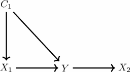
So we just modify the previous case to add this \(C_1\) variable with the following lines of code:

data["c_1"] = data.apply(lambda x: np.random.normal(0, 1) * x["environment"], axis=1)
data["x_1"] = data.apply(lambda x: x["c_1"] + np.random.normal(0, 1) * x["environment"], axis=1)
data["y"] = data.apply(lambda x: 1 * x["x_1"] + 0.5 * x["c_1"] + np.random.normal(0, 1), axis=1)

If we add \(C_1\) to the data frame, then we get:

>>> ICP(S_hat=array([0, 2]), q_values=array([1.02144993e-23, 1.00000000e+00, 3.97090776e-02]),
>>> p_value=2.6828782748093754)

So now it outputs, we should include the \(X_1\) and \(C_1\) to achieve invariance through the environments.

If we do not add it, then we have:

>>> ICP(S_hat=array([0, 1]), q_values=array([8.93818903e-40, 2.13782355e-05]),
>>> p_value=0.039709077611022575)

So \(X_1\) and \(X_2\) become the suggested causal variables, which is wrong.

Conclusion

ICP offers an exciting way to explore causal invariance in Machine Learning and helps build more robust models. At the same time, it suffers from the traditional problem of unmeasured confounders. However, it also presents other weaknesses that might avoid its usages, like the assumption of the same variance for the error in every environment, problems with highly correlated features, and difficulties in dealing with numerous input features.

References