Index
Introduction
The Time Robust Tree (TRT) 1 is a tree-based learning algorithm that uses timestamp information to learn splits that are optimal for time segments provided by the user, e.g., year. It means a split on a particular feature is only good if it works through all the years present in the data. The hypothesis is that splits that survive the time-test in the training set are more likely to survive it for future unseen periods. It was inspired by algorithms that explore invariance through environments to learn causal relationships. The test of time represents the invariance, while the time segments are the environments.
Something that bothered me while ensembling TRTs into a Time Robust Forest was the lack of randomization of its core design change: the time segmentation. In this post, I explore two alternatives to make it happen and test it on two datasets.
Randomizing the time segments
The code is available in the Time Robust Forest package, where code snippets on how to use it can be found in the readme. The experiments’ code was adapted from the previous design, and it is not that tidy, but they are available: GE News, Olist.
Enabling multiple time segments informed by the user
Previously, one could only inform a particular dataset segmentation considering the timestamp information. Either days, months, trimester, years, etc. The hypothesis is that mixing the invariance on different environment granularities can be more powerful. The model now accepts a set of columns representing different segmentations, and every new ensemble estimator will pick randomly from them.
The first practical advantage is ensembling the TRF with a Random Forest (RF) inside the same model since a segment column filled with 1s reproduces an RF. Beyond simply ensembling good models, one can have different availability of features through time. For example, a particular group of features did not exist three years ago. The current TRF does not deal well with these cases, but these features would be used in the RF estimators from the ensemble.
Random segments
Alternatively, the user can set a maximum number of splits, and the model will order the data according to time, create all the possible segmentations and select randomly from this set for every estimator in the ensemble.
Experiments
The design and optimal hyper-parameters from a previous setting were leveraged. The most important part is the data split: we first split using the time information. In-time set is for training and test, while out-of-time is for the holdout set. The same parameters were utilized, except for the number of estimators, which increased from 120 to 400 in all models. We will test the following models:
- Random Forest (benchmark): an RF, which is the TRF using a time column full of 1s;
- Time Robust Forest: a TRF using a single time column selected by the user;
- Random TRF (eng): a TRF using multiple time columns selected by the user;
- Random TRF (few): a TRF using a low value for maximum random segments;
- Random TRF (many): a TRF using a large value for maximum random segments;
- TRF + RF: a TRF using as time columns a time segment and a dummy column with no segment (RF);
GE News
The dataset 2 was expanded with more recent examples. In the table below, one of the Random TRF designs shows that the eng(inerred) could perform better than the previous challenger, which is the TRF. However, it was not explored how to select from the many options available for a Random TRF - would the Env K-folds select the best option? See the section “Hyper-parameter optimization” from this post.
| Model | Train AUC | Test AUC | Holdout AUC |
|---|---|---|---|
| Random TRF (eng) | .867 | .863 | .825 |
| Challenger | .870 | .866 | .822 |
| Random TRF (few) | .899 | .889 | .822 |
| TRF + RF | .905 | .893 | .821 |
| Benchmark | .919 | .898 | .813 |
| Random TRF (many) | .857 | .859 | .807 |
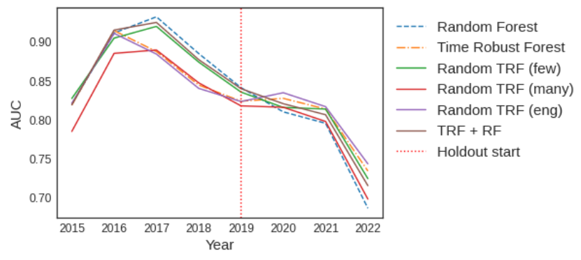
When we observe the performance over time, we see that the eng option during the in-time period is a shift of what we have for the challenger (Time Robust Forest). Nonetheless, when the holdout starts, they start to behave slightly differently. We see them inverting which model is performing better, just as challenger did with benchmark previously.
Is it a matter of simplicity?
Most of my skepticism about the TRF comes from the fact its design could be simply pushing the model to be simpler. The simplicity would go against overfitting, and it would generalize better. Even considering that in all the previous experiments, the model development pipeline follows standard practices for both benchmark and challenger, I like to keep challenging it.
To keep getting evidence it is not the case, I took the opportunity to train two simpler versions of the benchmark. First, I multiply the minimum number of examples by the number of distinct periods in the challenger model since it is the volume of total data the TRF demands to keep growing deeper. In the second case, I’ve forced the benchmark to have a similar training performance compared to the challenger. I did it by changing the minimum examples to split and the maximum depth.
The results in the image below show it might explain part of it. The simplified versions worsened the benchmark in the holdout. However, the models converge to the same performance after some years. Nonetheless, the simplified benchmark behavior is still very different from what we observed in the challenger. I wonder if the challenger would also converge if we had more data. The period is not sufficiently long to provide enough environments for the TRF to learn and let a very long holdout.

Olist
The Olist dataset 3 is not as voluminous as the GE News. We run ten bootstrap rounds to estimate model performance. I modified the previous optimal parameters by increasing the number of estimators from 140 to 240.
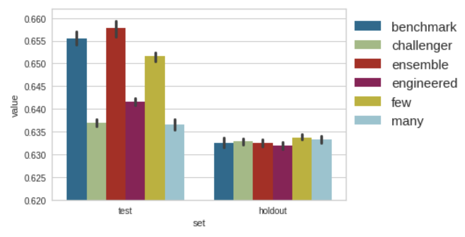
In the plot below, we can see the results for the test and holdout. As expected, when we ensemble the TRF with the RF, the test performance will go up. The same thing happens to the few case since it fragments the data guided by the time column, including the particular case of a single fragment. It is evidence the user should also control the minimum number of segments.
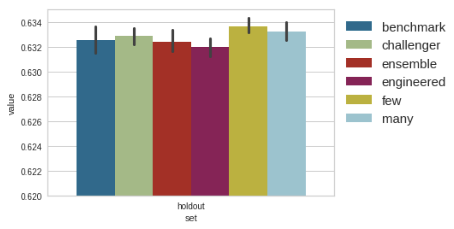
Since the performance in the holdout is very similar, we can zoom in. There is a lot of overlap in the intervals. However, it is interesting to notice how benchmark, challenger, ensemble, and engineered options are worse on average than few and many, which does not require expert knowledge on splitting the time information into meaningful segments.
Conclusion
The results are interesting in this minimal experimental setting. The GE News and the Olist dataset pointed to different approaches to creating the set of time segments to pick randomly from: engineered or randomly split. The GE dataset is large, but it needs to be challenged further. While the Olist results pretty much overlap. Segmenting the environment randomly goes against the idea of expert knowledge guiding the environment definition and assuming we’ll have data about it. One alternative to random selection is to make it part of the learning process or use data to guide it. A domain classifier is an excellent option to segment data periods that differ significantly. If we want to learn this split, we need to do it based on a criterion that is not a training error. The higher the segmentation, the higher the total minimum examples of splitting needed, the shallower the tree, and the simpler the model, the higher the training error. Unsupervised learning might make sense here too. Considering data from a certain period, look at how similar the following data segments are and define if we should consider them the same or a different environment based on a threshold or statistical test.
References
-
Moneda, L., & Mauá, D. (2022). Time Robust Trees: Using Temporal Invariance to Improve Generalization. BRACIS 2022. ↩
-
Moneda, L.: Globo esporte news dataset (2020), version 19. Retrieved July 11, 2022, from https://www.kaggle.com/lgmoneda/ge-soccer-clubs-news ↩
-
Sionek, A.: Brazilian e-commerce public dataset by olist (2019), version 7. Retrieved March 13, 2021, from https://www.kaggle.com/olistbr/brazilian-ecommerce ↩