Index

1. Introduction
2. Experiments
   1. Setup
   2. Performance
   3. The domain classifier
   4. Temporal views
   5. The hyper-parameters effect
   6. Feature importance
3. Conclusion

Introduction

This post contains a practical application of the Time Robust tree (TRT). To understand the model motivation, please read Introducing the Time Robust Tree - invariance in Machine Learning #3 or “Time Robust Trees: Using Temporal Invariance to Improve Generalization”¹. Most of our interest in this work is to reflect on dataset shift and generalization. However, in an industry setting, the Time Robust Forest (TRF), the ensemble version of the TRT, can offer an exciting challenger for settings one cannot retrain a model constantly.

We will explore some real-world datasets and compare the TRF to a Random Forest (RF). All the data and code for the experiments are available, just as the base package time-robust-forest.

The experiments

Setup

To validate the approach, seven public datasets in which a timestamp information and a reasonable time range are available were selected ^{2 3 4 5 6 7 8}.

We split every dataset into two time periods: training and holdout. Then training period data is split randomly between training and test. We use the Time Robust Forest python package for both benchmark and challenger.

The benchmark has all training examples with the same \(T_{period}\), which is a particular case the TRF becomes a regular Random Forest. The challenger uses yearly or year-monthly segments.

The hyper-parameter optimization uses an approach we identify as Environment K-Fold, which we explain in a previous post.

Performance

The first evidence we look for is a simple difference in performance. We hypothesize the TRF will not suffer as much as the RF to keep its performance in future unseen data, which we simulate with the Holdout set.

In the table below, it is possible to see the TRF did better in the holdout in three opportunities, while it is similar in two and loses in the other two.

This aggregated result is interesting, but looking further can help us understand how the TRF operates.

Dataset	Data split	Volume	Time range	RF	TRF	TRF-RF
GE News	Train	21k	2015-2018	.927	.865	-.062
	Test	5k	2015-2018	.879	.839	-.040
	Holdout	58k	2019-2021	.805	.821	.017
Kickstarter	Train	98k	2010-2013	.736	.717	-.019
	Test	24k	2010-2013	.705	.701	-.004
	Holdout	254k	2014-2017	.647	.661	.014
20 News	Train	8k	-	.939	.869	-.070
	Test	2k	-	.867	.828	-.039
	Holdout	8k	-	.768	.774	.006
Animal Shelter	Train	75k	2014-2017	.814	.803	-.011
	Test	19k	2014-2017	.792	.790	-.002
	Holdout	61k	2018-2021	.791	.791	.000
Olist	Train	41k	2017	.799	.695	-.104
	Test	10k	2017	.664	.641	-.023
	Holdout	62k	2018	.635	.635	.000
Chicago Crime	Train	100k	2001-2010	.936	.909	-.027
	Test	61k	2001-2010	.904	.899	-.005
	Holdout	90k	2011-2017	.905	.902	-.003
Building Permits	Train	90k	2013-2015	.990	.984	-.006
	Test	22k	2013-2015	.974	.972	-.002
	Holdout	193k	2011-2017	.977	.973	-.004

The domain classifier

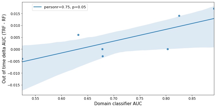
In the previous table, it is possible to verify that the cases where TRF is an exciting challenger are the ones in which the benchmark has problems performing in the holdout as well as in the test. We train a domain classifier using the holdout as the target to clarify the evidence under scenarios the future data changes the most. The higher the AUC, the more significant the difference between test and holdout in that dataset. As seen in the figure below, the results show that the TRF performed better in the datasets with a more remarkable shift between training and holdout data.

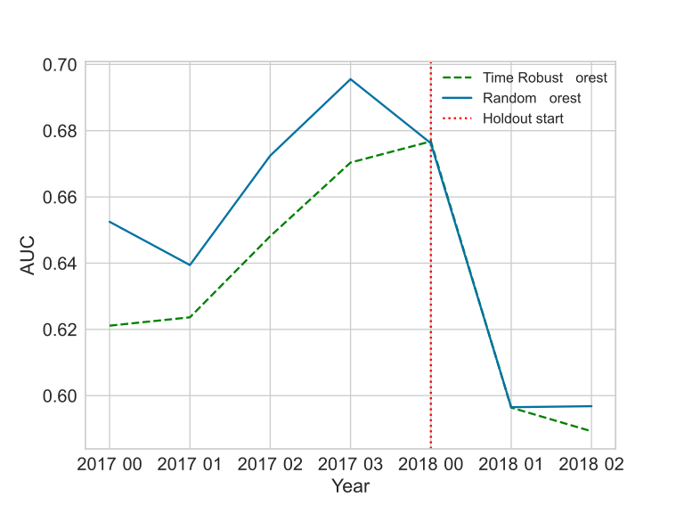
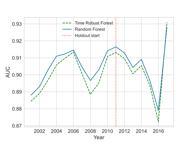
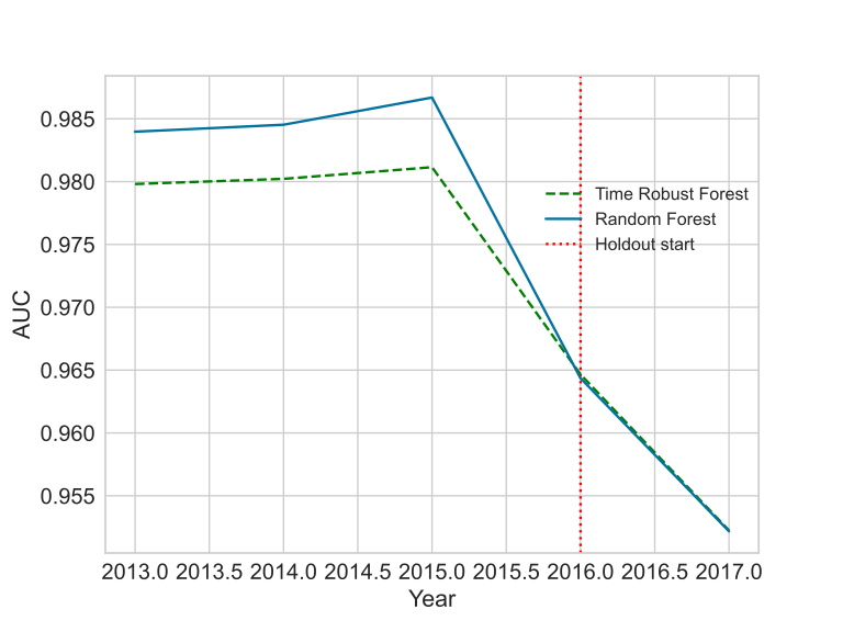
Temporal views

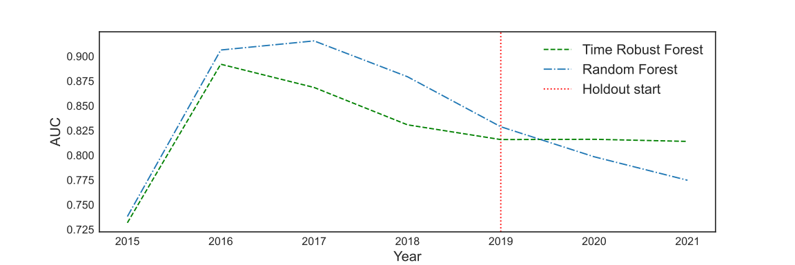
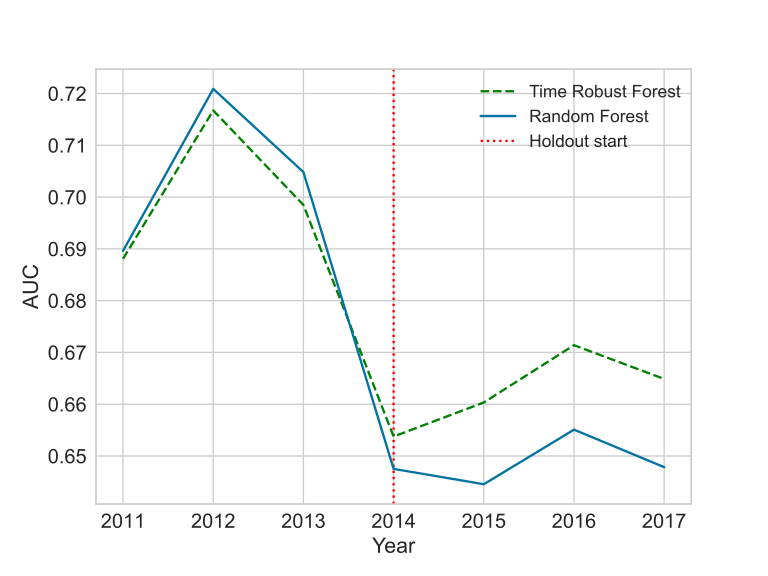
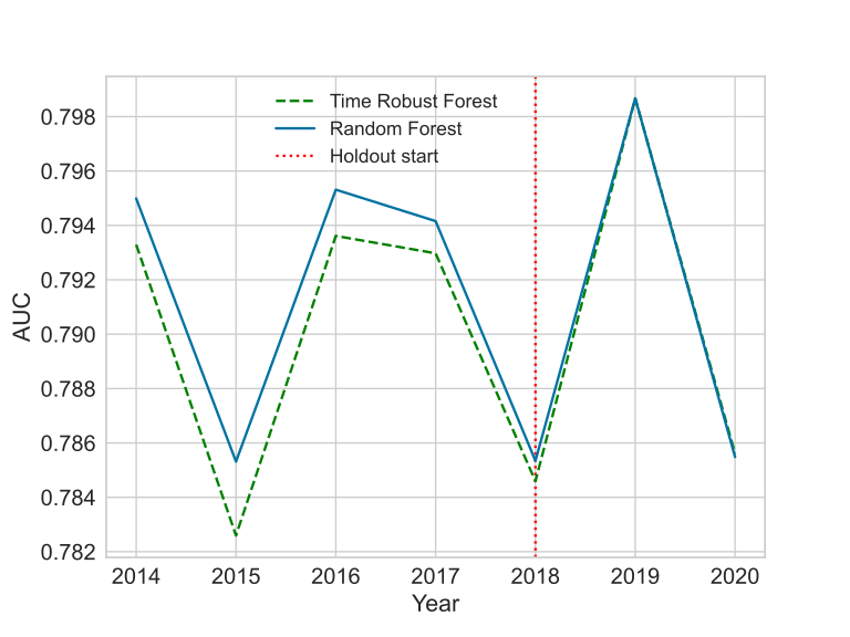
The hypothesis is that TRF would be able to learn more stable relationships, which would exclude spurious relationships. These relationships would not degrade as quickly as the others. We have a hint from the aggregated performance metric from the previous table, but we want to see it over time.

The most interesting case is the GE News. Notice how the curve shape is different during the holdout. In the other cases, the parallel shift seems to be evidence of a different model capacity. Still, if the setup is close enough to normal model development, the results put the TRF as a reasonable challenger for the RF.

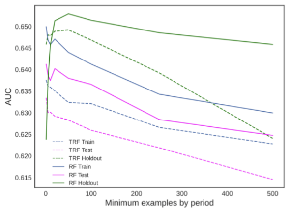
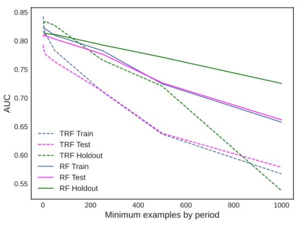
The hyper-parameters effect

Though we optimize both of the models with a similar procedure, the chances are that hyper-parameters can produce misleading results. The parameter we care about the most on the TRF is the minimum number of examples from each period. In the RF, the similar parameter is the minimum number of examples to split. To verify how this parameter influenced the results, we fixed all the others and let this one change.

As we can see in the images below, it was a matter of parametrization in the Kickstarter case, while in GE News, it was not. The dashed lines represent the TRF, while the green curves are about the holdout sets. We can see the RF has the power to solve the Kickstarter with a higher holdout performance, while in GE News, the dashed green curve goes to a level the continuous one does not reach.

Feature importance

If the TRF was to select stable relationships, we expect that the features would assume different importance. However, in terms of the order, there was little difference. The only pattern we could identify was that the TRF concentrated importance on the top features in the cases it outperformed the RF.

In the table below, we can see the feature importance of the GE News dataset. Notice how importance the TRF concentrates on the top features and how the importance quickly decreases as we go to the less important ones.

RF		TRF
Feature	Importance	Feature	Importance
atleta	0.043446	atleta	0.090731
cada	0.034933	sabe	0.036755
partidas	0.019544	cada	0.034831
primeiro	0.014367	partidas	0.021660
sabe	0.012230	lateral	0.016985
dia	0.010441	chegar	0.015238
cinco	0.009303	dia	0.012248
lateral	0.006325	cinco	0.011322
video	0.006182	camisa	0.006628
rodrigo	0.005493	precisa	0.006192
defesa	0.004620	globoesport	0.004892
globoesporte	0.004507	defesa	0.004150
precisa	0.004204	todos	0.003037
momento	0.003925	possível	0.002211
treinador	0.003699	lesão	0.001797
camisa	0.003505	video	0.001595
hoje	0.003442	vitória	0.001177
difícil	0.003328	dentro	0.000943
possível	0.003327	neste	0.000874
todos	0.003132	nova	0.000581

Conclusion

In most cases, the TRF looks like regularization since it has worse training performance and a better holdout result. In these cases, the shape of the curve in the holdout is similar for the RF and the TRF. However, it might be the case that in most datasets, the low number of features does not enable it to find stability from a particular source. The most interesting case is also the one with the highest number of features, which is GE News. The interestingness of this case is that it provides evidence that phenomena we want to predict could be composed of many concepts, which change at different rates as time passes. At the same time, models cannot capture this nuance and tend to focus on simple and spurious relationships.

Nonetheless, the domain classifier points to a simple way to find a reason to try the TRF for a particular problem, and its performance does not lose by far in the cases it loses to the RF.

References

		
		  @article{moneda2022trtexp-blogpost,
		  author = {Moneda, Luis},
		  title = Time Robust Tree experiments on real datasets,
		  journal = {Blogpost at lgmoneda.github.io},
		  year = {2022},
		  howpublished = {\url{lgmoneda.github.io}},
		  }