Index

1. Introduction
2. The data
3. Modeling
4. Selecting temporally stable features
5. All features (benchmark) Vs Stable features (challenger)

Introduction

SHAP values can be seen as a way to estimate the feature contribution to the model prediction. We can connect the fact the feature is contributing to it to the importance it has. The larger the contribution, the larger the importance - there are some caveats, but let’s keep it simple.

One common strategy to select features is to use their average contribution and add them to the model while looking to a validation set performance change. Once we hit the “elbow”, a place in the curve with enough gain, we stop adding, and we end up reducing the number of features.

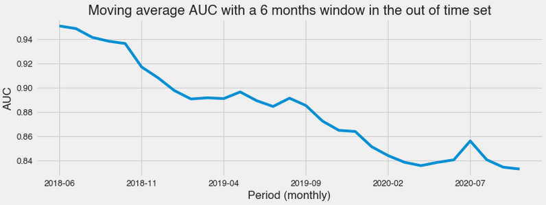
But once we have temporal information in the data, we can do it differently. We don’t want a model to only perform well in general unseen data. We hope it performs nicely in the unseen and future, which is susceptible to different types of Dataset shift. We can try to incorporate this requirement into the model design process. Generally, models degrade over time, as we see in the following plot.

The data

We’re going to use the GE soccer clubs news dataset, which I have extracted from the GE website and organized. In short, it’s a set of sports articles about soccer clubs. Since it was extracted from every club section, it can be used as a label in a task of identifying based on the text which club the article is about. You can find an explanation about it on the dataset Kaggle page. We will make it a binary classification problem by picking Flamengo as the positive case. All code for our experiment can be seen here.

If it is interesting for you, please upvote it on Kaggle to give it visibility.

The dataset choice was based on the fact that it has a time range so we can observe model performance being challenged by the proof of time.

Modeling

The focus here is not on building state of the art solution for a binary classification natural language processing problem but the feature selection process. Here the vocabulary is truncated at 1000 words. We use some stop words, tf-idf, 1-gram, lightgbm, exclude the club name from the article text, and that’s it.

Selecting temporally stable features

Our definition of temporal stability is related to the variance of the importance of a particular feature considering different time slices. In this case, we’re going to slice time in months. So we simply calculate the feature importance for every month and check its variance.

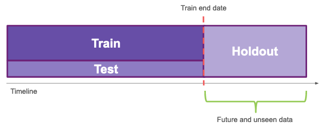
To do it, we split our dataset into three sets: train, test, and holdout. The first two sets are “in time”, they go from 2015-06 until 2018-01 (the train end date), the holdout is “out of time”, it goes from 2018-01 until 2020-11 (the most recent data we have).

After training an auxiliary model using the train data, we store feature importance for every month in the in-time period and calculate its average and variance. The average shap value is called contribution, and the variance is called instability here. Using some arbitrary threshold for both, we divide the features into four groups that combine high and low contribution and high and low instability, as we can see in the following image.

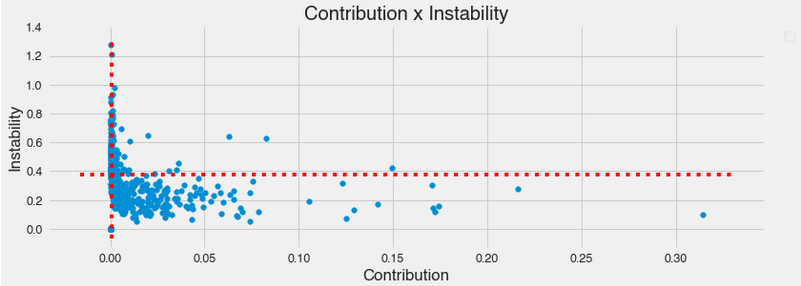
The central argument here is that if we want to prefer features, we should pick the high-contribution and low-instability group since it’s reasonable to imagine its predictive power is more likely to show robustness to future changes than the high-contribution and high-instability ones.

All features (benchmark) Vs Stable features (challenger)

To make sure hyper-parameters were reasonably adjusted, we use Pycaret, an automl library, which uses k-fold, including all in-time data.

The same vectorizer used for the feature selection, fitted in the train data, is used for both models. However, one includes all the 1000 features, while the other contains only 414 features.

We calculate the AUC, an ordering metric, for every month present in the in-time period and the out of time to evaluate the models. In the in-time period, it’s the test performance, while in the out-of-time, it’s the holdout performance.

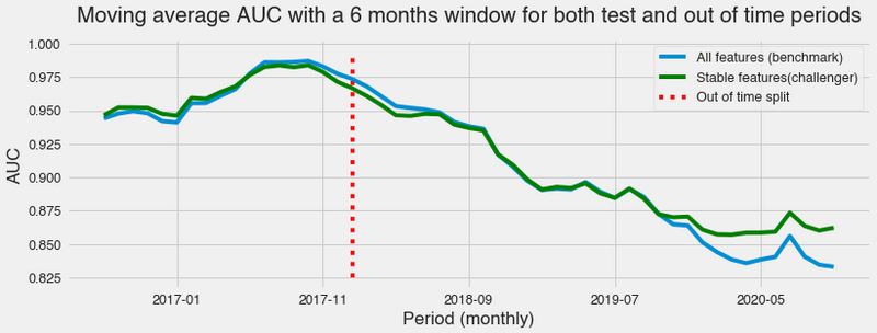
Both models have a similar performance during the in-time period, and we can say that at its end and the beginning of the out-of-time split, the benchmark does better. Then, they perform the same way until far in the future, when the benchmark starts to degrade faster than the stable features model.

This is evidence that using temporal stability as a criterion for feature selection can improve the model’s robustness regarding unknown shifts in the data behavior. Of course, it’s minimal evidence since bootstrapping, different modeling approaches, and diverse datasets and tasks could reveal the approach does not consistently address the problem. But considering the real-world data nature, the volume of articles, and the reasonable time range, it’s an exciting result.