Index
- Introduction
- Unit Selection problem
- Counterfactual formulation of Unit Selection Problem
- The example
Introduction
I’ve read some parts of Unit Selection Based on Counterfactual Logic1. Unit selection is the task of selecting individuals who respond to a specific treatment. I had to go through the calculation of one of the examples to convince myself I understood the work. It is the calculation of the proposed objective function using counterfactual logic. So I’m sharing it to support other people doing the same.
I recommend reading Ang Li’s thesis since I’ll briefly expose a few concepts from it.
Unit Selection problem
The individual benefit varies accordingly to their compliance type: always-takers, never-takers, compliers, and defiers.
The classical way to solve this problem is to run an A/B test, then use the characteristics \(C\) we have about the customers to predict heterogeneous treatment effects and select only the compliers.
A/B test heuristics for decision making
There are two classical objective functions to decide on applying action \(a\) to incentivize behavior \(r\).
The first checks if doing action \(a\) makes people respond \(r\) more:
\[\begin{align} \begin{split} Obj_{1} = argmax_{c} 100 \times P(r \mid c, do(a)) - 100 \times P(r \mid c, do(a')) \end{split}\label{eq:obj_1} \end{align}\]The second contrasts the benefit of response \(r\) under the action \(a\), minus the outcome behaving as \(r\) without the action \(a\).
\[\begin{align} \begin{split} Obj_{2} = argmax_{c} 100 \times P(r \mid c, do(a)) - 140 \times P(r \mid c, do(a')) \end{split}\label{eq:obj_2} \end{align}\]Counterfactual formulation of Unit Selection Problem
Li (2021) shows that the previous heuristics fail and propose an objective function based on counterfactual logic.
See Theorem 4. Consider the benefits of offering the treatment to compliers (\(\beta\)), always-taker (\(\gamma\)), never-taker (\(\theta\)), and defier (\(\delta\)), a \(c\) representing the characteristics of the individuals, or simply subgroups. The only condition is that the \(C\) do not contain any descendant of the encouragement \(X\).
\[\begin{align} \begin{split} argmax_{c} \beta P(\text{complier} \mid c) + \gamma P(\text{always-taker}\mid c) + \theta P(\text{never-taker}\mid c) + \delta P(\text{defier}\mid c) \end{split}\label{eq:counter_f} \end{align}\]Using \(a\) to denote taking action and \(a'\) its absence, we have, in terms of probabilities of sufficiency and necessity:
\[argmax_{c} \beta P(r_a, r'_{a'} \mid c) + \gamma P(r_{a}, r_{a'} \mid c) + \theta P(r'_a, r'_{a'ƒ}\mid c) + \delta P(r'_{a}, r_{a'}\mid c)\]This case requires observational and experimental data (more details below).
If we observe either Gain equality or Causal monotonicity, it becomes simpler:
\[(\beta - \theta) P(y_x \mid c) + (\gamma - \beta)P(y_{x'} \mid c) + \theta\]With do notation:
\[(\beta - \theta) P(r \mid do(a)) + (\gamma - \beta)P(r \mid do(a')) + \theta\]In this last case, we can estimate it with only experimental data.
Gain Equality
Define a benefit vector of applying the treatment in the compliance groups following: compliers (\(\beta\)), always-taker (\(\gamma\)), never-taker (\(\theta\)), and defier (\(\delta\)). We say it satisfies the gain equality if:
\[\beta + \delta = \gamma + \theta\]Causal monotonicity
Causal monotonicity of a variable \(Y\) in respect to a variable \(X\) means:
\[y'_{x} \text{ AND } y_{x'} = \text{false}\]If treatment \(x\) does not make the expected outcome \(y\), the lack of it won’t make it happen.
The general case
The proposed function Objective Function \ref{eq:counter_f} is bounded as follows:
\[\begin{align} \begin{split} {}& max\{p_1, p_2, p_3, p_4\} \leq f \leq min\{p_5, p_6, p_7, p_8\} \text{ if } \sigma < 0, \\ {}& max\{p_5, p_6, p_7, p_8\} \leq f \leq min\{p_1, p_2, p_3, p_4\} \text{ if } \sigma > 0, \\ \end{split} \end{align}\]Where
\[\begin{align} \begin{split} {}& \sigma = \beta - \gamma -\theta + \delta \\ {}& p_1 = (\beta - \theta)P(y_x\mid c) + \delta P(y_{x'}\mid c) + \theta P(y'_{x'}\mid c), \\ {}& p_2 = \gamma P(y_x\mid c) + \delta P(y_{x'}\mid c) + (\beta - \gamma) P(y'_{x'}\mid c), \\ {}& p_3 = (\gamma - \delta)P(y_x\mid c) + \delta P(y_{x'}\mid c) + \theta P(y'_{x'}\mid c) + (\beta - \gamma - \theta + \delta)[P(y, x \mid c) + P(y', x' \mid c)], \\ {}& p_4 = (\beta - \theta)P(y_x\mid c) - (\beta - \gamma - \theta)P(y_{x'}\mid c) + \theta P(y'_{x'}\mid c) + (\beta - \gamma - \theta + \delta)[P(y, x' \mid c) + P(y', x \mid c)], \\ {}& p_5 = (\gamma - \delta)P(y_x\mid c) + \delta P(y_{x'}\mid c) + \theta P(y'_{x'}\mid c), \\ {}& p_6 = (\beta - \theta)P(y_x\mid c) - (\beta - \gamma - \theta)P(y_{x'}\mid c) + \theta P(y'_{x'}\mid c), \\ {}& p_7 = (\gamma - \delta)P(y_x\mid c) - (\beta - \gamma - \theta)P(y_{x'}\mid c) + \theta P(y'_{x'}\mid c) + (\beta - \gamma - \theta + \delta)P(y \mid c), \\ {}& p_8 = (\beta - \theta)P(y_x\mid c) + \delta P(y_{x'}\mid c) + \theta P(y'_{x'}\mid c) - (\beta - \gamma - \theta + \delta)P(y \mid c), \\ \end{split}\label{eq:ps} \end{align}\]No observational data case
We can exclude the terms containing observational probabilities and use:
\[\begin{align} \begin{split} {}& max\{p_1, p_2\} \leq f \leq min\{p_3, p_4\} \text{ if } \sigma < 0, \\ {}& max\{p_3, p_4\} \leq f \leq min\{p_1, p_2\} \text{ if } \sigma > 0, \\ \end{split}\label{eq:simple_ps} \end{align}\]The \(p_1, p_2\) are the same. But \(p_3, p_4\) now are the \(p_5, p_6\) from \ref{eq:ps}.
The example
It is the example in section 5.3.1. In summary, we want to evaluate an action to avoid customer churn. We offer a discount to renew a subscription. The outcome of the action is considered as \$100 for compliers (\$140 profit less \$40 cost), -\$60 for always takers (-\$40 discount and an extra -\$20 since they may require additional discounts in the future), \$0 for never taker, and -\$140 for a defier since the company loses the customer. The discount is applied to two groups of customers identified by \(c\).
I’ll just expose the case for group 1 since it is similar to group 2.
Here’s the A/B testing result:
| A/B test result | do(a) | do(a') | |
|---|---|---|---|
| Group 1 | r | 262 | 175 |
| Group 1 | r' | 88 | 175 |
| Group 2 | r | 87 | 52 |
| Group 2 | r' | 263 | 298 |
Let’s start with the A/B test heuristics.
To use Objective function \ref{eq:obj_1}, we need the following probabilities estimated from the A/B test:
\[P(r \mid c, do(a)) = \frac{262}{262+88} = 0.7485 \\ P(r \mid c, do(a')) = \frac{175}{175+175} = 0.5 \\\]Replacing in the equation:
\[Obj_{1} = 100 \times 0.7485 - 100 \times 0.5 = 24.85 =^{~} 25\]For the Objective function \ref{eq:obj_2}, we need the same probabilities, but we weight it differently:
\[Obj_2 = 100 \times 0.7485 - 140 \times 0.5 = 4.857 =^{~} 4.86\]Now we estimate the proposed objective function. We first analyze the benefit vector:
\[\sigma = \beta - \gamma -\theta + \delta = 100 - (-60) - 0 + (-140) = 20\]Gain equality is not respected. Since \(\sigma > 0\), we would use the set of Equations \ref{eq:ps}. However, since in this example we only have experimental data, we need to use \ref{eq:simple_ps}.
We start by exposing the components:
\[p(y_x \mid c) = \frac{262}{262+88} = 0.785 \\ p(y_{x'} \mid c) = \frac{175}{175+175} = 0.5 \\ p(y'_{x'} \mid c) = \frac{175}{175+175} = 0.5 \\ p(y'_x \mid c) = \frac{88}{262+88} = 0.2414 \\\] \[\begin{align} \begin{split} {}& p_1 = (\beta - \theta)P(y_x\mid c) + \delta P(y_{x'}\mid c) + \theta P(y'_{x'}\mid c) \\ {}& p_1 = (100 - 0)\times 0.7485 + (-140) \times 0.5 + 0 \times 0.5 \\ {}& p_1 = 4.85 \\ \\ {}& p_2 = \gamma P(y_x\mid c) + \delta P(y_{x'}\mid c) + (\beta - \gamma) P(y'_{x'}\mid c) \\ {}& p_2 = -60 \times 0.740815 + (-140) \times 0.2514 + (100 - (-60)) \times 0.5 \\ {}& p_2 = -0.106 \\ \\ {}& p_3 = (\gamma - \delta)P(y_x\mid c) + \delta P(y_{x'}\mid c) + \theta P(y'_{x'}\mid c) \\ {}& p_3 = (-60 - (-140)) \times 0.7485 + (-140) \times 0.5 + 0 \times 0.5 \\ {}& p_3 = -10.12\\ \\ {}& p_4 = (\beta - \theta)P(y_x\mid c) - (\beta - \gamma - \theta)P(y_{x'}\mid c) + \theta P(y'_{x'}\mid c), \\ {}& p_4 = (100 - 0 \times 0.7485 - (100 - (-60) - 0) \times 0.5 + 0 \times 0.5 \\ {}& p_4 = -5.15 \\ \end{split} \end{align}\]We end up with:
\[\begin{align} \begin{split} max\{-10.12, -5.15\} \leq {}& f \leq min\{4.85, -0.106\} \\ -5.15 \leq {}& f \leq -0.106 \\ \end{split} \end{align}\]We use the midpoint of -5.15 and -0.106, which is -2.63. And that’s what we have in table 5.2 (Li, 2021).
Li provides the proportion of compliance types in group 1, which is never known.
| Complier | Always-taker | Never-taker | Defier | |
|---|---|---|---|---|
| Group 1 | 30% | 45% | 20% | 5% |
When we estimate the expected value of applying the discount on them:
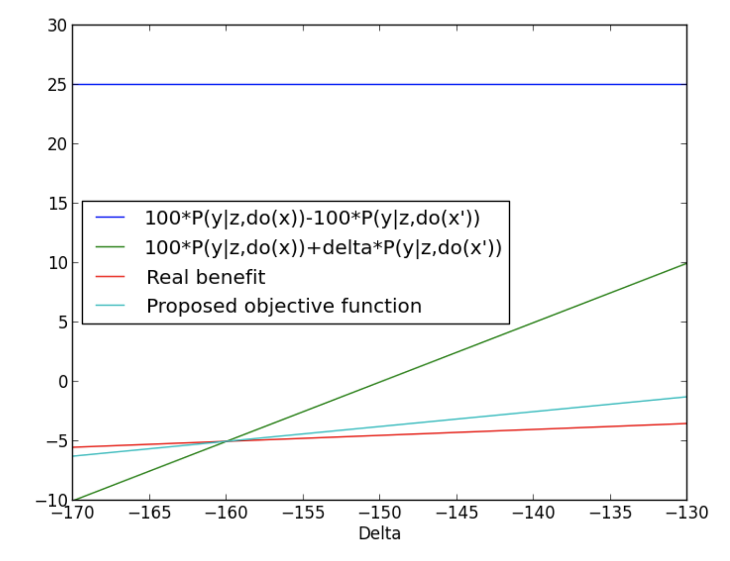
\[\begin{align} \begin{split} {}& E[\text{profit}] = \beta P(\text{complier} \mid c=1) + \gamma P(\text{always-taker}\mid c=1) + \theta P(\text{never-taker}\mid c=1) + \delta P(\text{defier}\mid c=1)\\ {}& E[\text{profit}] = 100 \times 0.3 -60 \times 0.45 + 0 \times 0.2 -140 \times 0.05 \\ {}& E[\text{profit}] = -4 \\ \end{split} \end{align}\]We realize how \(f_3\) is a better estimate of it. Li provides a plot on how the actual value and the three functions estimates change as we change \(\delta\).
References
-
Li, A. (2021). Unit selection based on counterfactual logic. : University of California, Los Angeles. ↩